건축 설계의 초기 단계에서는 건물이 배치될 방향에 대한 축이라는 개념이 있습니다. 이는 건물의 기능성, 심미성, 환경 조건을 고려한 최적의 배치를 결정하는 데 중요한 역할을 합니다. 이 프로젝트의 목표는 주어진 2D 다각형을 몇 개의 축으로 분할해야 하는지와 어떻게 분할할지를 결정할 수 있는 모델을 개발하는 것입니다.
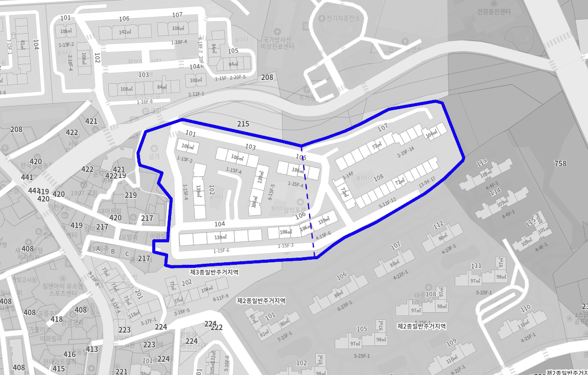
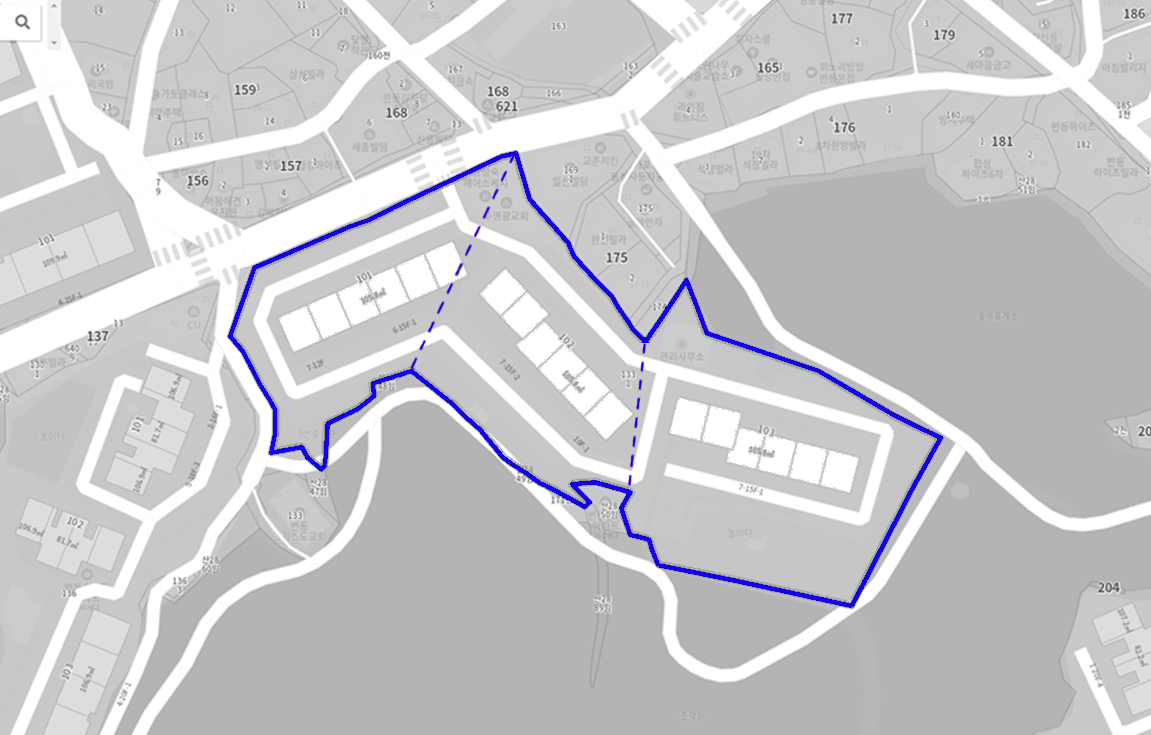
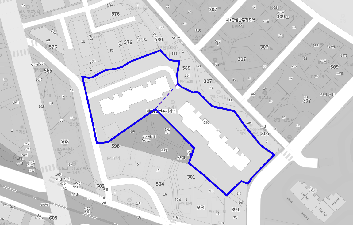
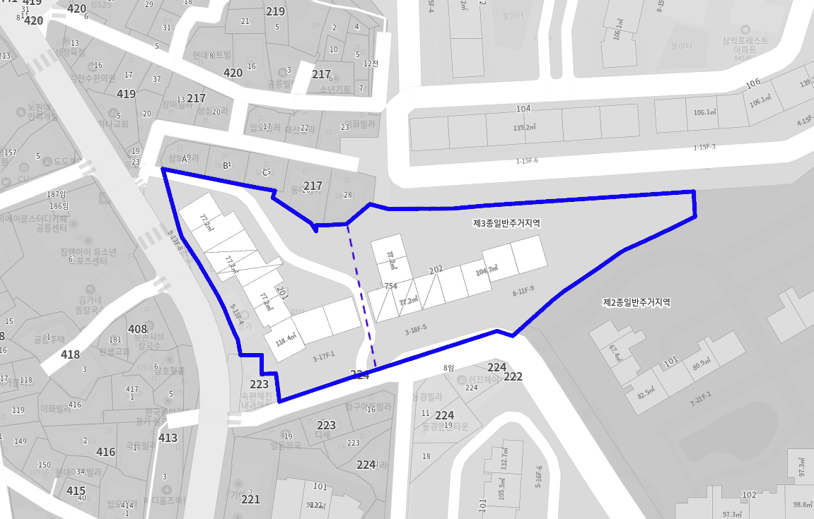
Segmented lands by a human architect
위 그림들은 건축가가 임의로 설정한 가상의 분할선입니다. 그림에서 아파트들은 분할된 다각형을 기반으로 배치되어 있습니다. 건축가들은 주어진 2D 다각형을 몇 개의 축으로 분할해야 하는지와 어떻게 분할할지를 직관적으로 알고 있지만, 이러한 직관을 컴퓨터에게 설명하는 것은 어렵습니다.
이를 달성하기 위해, 저는 딥러닝과 그래프 이론을 결합하여 사용할 것입니다. 그래프에서 다각형의 각 점은 노드가 되고 점들 간의 연결은 엣지가 됩니다. 이 개념을 바탕으로, 주어진 다각형을 최적으로 분할하는 방법을 학습하는 GNN 기반 모델을 구현할 것입니다.
A simple understanding of graph and GNN
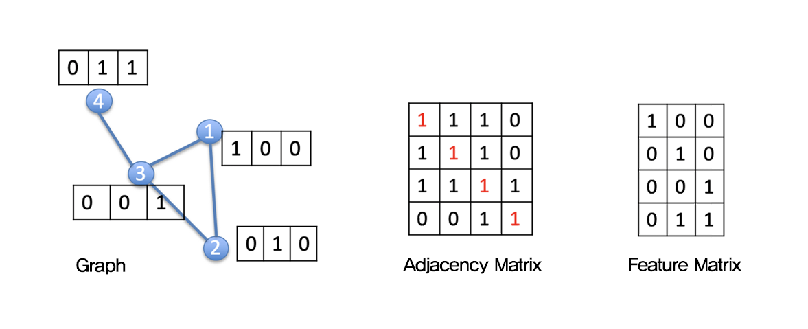
데이터를 생성하기 전에, 그래프와 그래프 신경망에 대해 이해해 보겠습니다. 기본적으로 그래프는 \( G = (V, E) \)로 정의됩니다. 이 표현에서 \( V \)는 정점(노드)의 집합이고 \( E \)는 엣지의 집합입니다.
그래프는 주로 Adjacency Matrix로 표현됩니다. 점의 개수가 \( n \)일 때, Adjacency Matrix \( A \)의 크기는 \( n \times n \)입니다. 머신러닝에서 그래프를 다룰 때는 점들의 특성을 나타내는 Feature Matrix 표현됩니다. 특성의 개수가 \( f \)일 때, Feature Matrix \( X \)의 차원은 \( n \times f \)입니다. Understanding of the graph expression In this figure, \( n = 4 \), \( f = 3 \) \( A = n \times n = 4 \times 4 \) \( X = n \times f = 4 \times 3 \).
그래프는 다양한 분야에서 데이터를 표현하는 데 사용되며, 다음과 같은 이유로 딥러닝 모델에 기하학을 가르칠 때 유용합니다:
Representing Complex Structures Simply: 그래프는 복잡한 구조와 관계를 효과적으로 표현하여 다양한 형태의 기하학적 데이터를 모델링하는 데 적합합니다.
Flexibility: 그래프 데이터구조는 다양한 수의 노드와 엣지를 수용할 수 있어, 다양한 형태와 크기의 객체를 다룰 때 유리합니다.
Graph Neural Network(GNN)은 그래프 구조에서 동작하도록 설계된 신경망의 한 종류입니다. 벡터나 행렬과 같은 고정된 크기의 입력에서 작동하는 전통적인 신경망과 달리, GNN은 크기와 연결성이 가변적인 그래프 구조의 데이터를 처리할 수 있습니다. 이러한 특성으로 인해 GNN은 소셜 네트워크, Geometry 등과 같이 관계가 중요한 작업에 특히 적합합니다. GNN은 주로 연결과 이웃 노드들의 상태를 사용하여 각 노드의 상태를 업데이트(학습)합니다(Message Passing). 그런 다음 최종 상태를 기반으로 예측이 이루어집니다. 이 최종 상태는 일반적으로 Node Embedding이라고 합니다(또는 노드의 원시 특성이 다른 표현으로 변환되기 때문에 Encoding이라고도 할 수 있습니다).
Message Passing에는 다양한 방법이 있지만, 이 작업은 기하학을 다루게 될 것이므로 Spatial Convolutionan Network를 기반으로 한 모델에 집중해 보겠습니다. 이 방법은 중요한 기하학적 및 공간적 구조를 가진 데이터를 표현하는 데 적합한 것으로 알려져 있습니다. 공간 합성곱 네트워크를 사용하는 GNN은 각 노드가 이웃 노드들의 정보를 통합할 수 있게 하여 지역적 특성을 더 정확하게 이해할 수 있게 합니다. 이를 통해 모델은 기하학의 복잡한 형태와 특성을 더 잘 이해할 수 있습니다. Convolution operations From the left, 2D Convolution · Graph Convolution
Spatial Convolutional Network (SCN)의 아이디어는 Convolutional Neural Network (CNN)와 유사합니다. 이미지는 grid-shaped graph로 변환될 수 있습니다.
CNN은 필터를 사용하여 중심 픽셀의 주변 픽셀들을 결합하여 이미지를 처리합니다. SCN은 이 아이디어를 그래프 구조로 확장하여, 주변 픽셀 대신 연결된 이웃 노드들의 특성을 결합합니다. 구체적으로, CNN은 필터가 각 픽셀의 주변 영역을 고려하여 특성을 추출하는 규칙적인 격자 구조에서 이미지를 처리하는 데 유용합니다. 반면에, SCN은 일반적인 그래프 구조에서 작동하며, 각 노드의 특성을 연결된 이웃들의 특성과 결합하여 Embedding을 생성합니다.
Data preparation
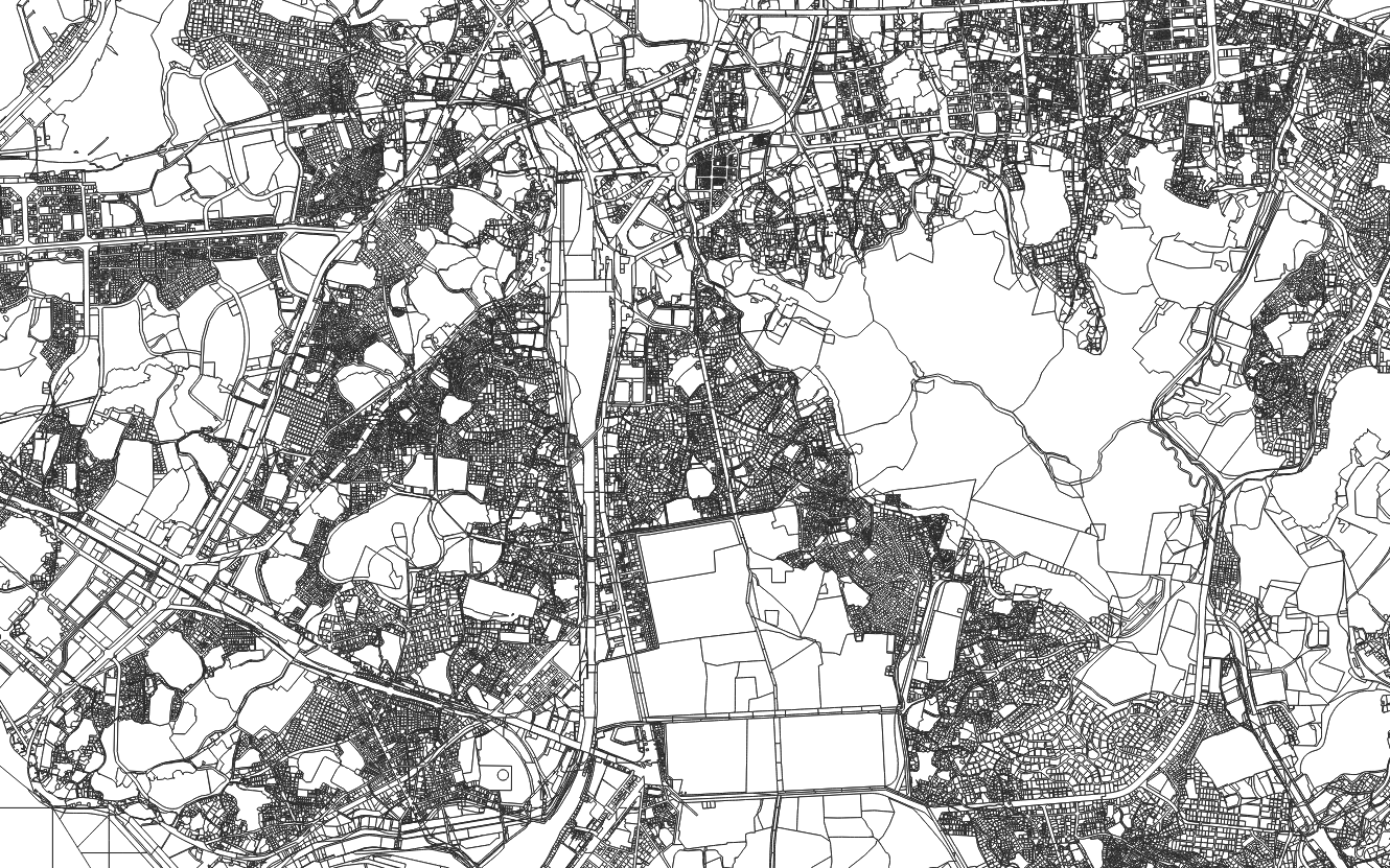
위에서 그래프와 GNN에 대해 간단히 살펴보았으니, 이제 데이터를 준비해 보겠습니다! 우리 주변에는 이미 많은 원시 다각형이 있으며, 그것이 바로 토지입니다. 먼저, vworld에서 원시 다각형을 수집해 보겠습니다. 아래는 제가 vworld에서 수집한 모든 원시 다각형의 일부입니다.
Somewhere in Seoul.shp
이제 raw polygons을 수집했으니, feature matrix에 포함될 polygon의 특성들을 정의해 보겠습니다. 다음과 같습니다:
X coordinate (normalized)
Y coordinate (normalized)
Inner angle of each vertex (normalized)
Incoming edge length (normalized)
Outgoing edge length (normalized)
Concavity or convexity of each vertex
Minimum rotated rectangle ratio
Minimum rotated rectangle aspect ratio
Polygon area
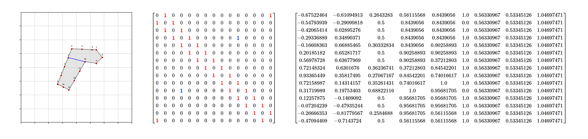
그런 다음, 이러한 데이터를 graph 형태로 변환해야 합니다. 다음은 수작업 라벨링의 예시입니다: Land polygon in Gangbukgu, Seoul From the left, raw polygon & labeled link · adjacency matrix · feature matrix
하지만 수많은 raw polygons을 수작업으로 라벨링하는 것은 불가능하기 때문에, 이 데이터를 자동으로 생성해야 합니다. 알고리즘으로 완전 자동화할 수 있다면 좋겠지만, 그것이 가능하다면 딥러닝이 필요하지 않았을 것입니다 🤔. 그래서, 수작업을 조금이라도 줄일 수 있는 간단한 알고리즘을 개발했습니다. 이 알고리즘은 다각형의 triangulations에서 영감을 받았습니다. 이 알고리즘의 과정은 다음과 같습니다:
Triangulate a polygon: Triangulation edge들을 추출합니다.
Generate Splitter Combinations: 반복 처리를 위한 모든 가능한 분할선 조합을 생성합니다.
Iterate Over Combinations: 최적의 분할된 다각형을 찾기 위해 모든 가능한 분할선 조합을 반복합니다.
Check Split Validity: 모든 분할이 유효한지 확인합니다.
Compute Scores and evaluation: 최적의 분할을 저장하기 위한 점수를 계산합니다.
다섯 번째 단계에서 사용되는 점수들(even_area_score, ombr_ratio_score, slope_similarity_score)은 다음과 같이 계산되며, 각 점수는 가중 합으로 집계되어 가장 낮은 점수를 가진 segmentation을 얻습니다.
이 알고리즘의 전체 코드는 여기에서 확인할 수 있으며, 알고리즘의 핵심 부분은 다음과 같습니다.
    def segment_polygon(
        self,
        polygon: Polygon,
        number_to_split: int,
        segment_threshold_length: float,
        even_area_weight: float,
        ombr_ratio_weight: float,
        slope_similarity_weight: float,
        return_splitters_only: bool = True,
    ):
        """Segment a given polygon

        Args:
            polygon (Polygon): polygon to segment
            number_to_split (int): number of splits to segment
            segment_threshold_length (float): segment threshold length
            even_area_weight (float): even area weight
            ombr_ratio_weight (float): ombr ratio weight
            slope_similarity_weight (float): slope similarity weight
            return_splitters_only (bool, optional): return splitters only. Defaults to True.

        Returns:
            Tuple[List[Polygon], List[LineString], List[LineString]]: splits, triangulations edges, splitters
        """

        _, triangulations_edges = self.triangulate_polygon(
            polygon=polygon,
            segment_threshold_length=segment_threshold_length,
        )

        splitters_selceted = None
        splits_selected = None
        splits_score = None

        for splitters in list(itertools.combinations(triangulations_edges, number_to_split - 1)):
            exterior_with_splitters = ops.unary_union(list(splitters) + self.explode_polygon(polygon))

            exterior_with_splitters = shapely.set_precision(
                exterior_with_splitters, self.TOLERANCE_LARGE, mode="valid_output"
            )

            exterior_with_splitters = ops.unary_union(exterior_with_splitters)

            splits = list(ops.polygonize(exterior_with_splitters))

            if len(splits) != number_to_split:
                continue

            if any(split.area < polygon.area * 0.25 for split in splits):
                continue

            is_acute_angle_in = False
            is_triangle_shape_in = False
            for split in splits:
                split_segments = self.explode_polygon(split)
                splitter_indices = []

                for ssi, split_segment in enumerate(split_segments):
                    if split_segment.length <= self.TOLERANCE_LARGE * 2:
                        continue

                    reduced_split_segment = DataCreatorHelper.extend_linestring(
                        split_segment, -self.TOLERANCE_LARGE, -self.TOLERANCE_LARGE
                    )
                    buffered_split_segment = reduced_split_segment.buffer(self.TOLERANCE, cap_style=CAP_STYLE.flat)

                    if buffered_split_segment.intersects(MultiLineString(splitters)):
                        splitter_indices.append(ssi)
                        splitter_indices.append(ssi + 1)

                degrees = self.compute_polyon_inner_degrees(split)
                degrees += [degrees[0]]

                if (np.array(degrees)[splitter_indices] < 20).sum():
                    is_acute_angle_in = True
                    break

                if len(self.explode_polygon(self.simplify_polygon(split))) == 3:
                    is_triangle_shape_in = True
                    break

            if is_acute_angle_in or is_triangle_shape_in:
                continue

            sorted_splits_area = sorted([split.area for split in splits], reverse=True)
            even_area_score = (sorted_splits_area[0] - sum(sorted_splits_area[1:])) / polygon.area * even_area_weight

            ombr_ratio_scores = []
            slope_similarity_scores = []

            for split in splits:
                ombr = split.minimum_rotated_rectangle
                each_ombr_ratio = split.area / ombr.area
                inverted_ombr_score = 1 - each_ombr_ratio
                ombr_ratio_scores.append(inverted_ombr_score)

                slopes = []
                for splitter in splitters:
                    if split.buffer(self.TOLERANCE_LARGE).intersects(splitter):
                        slopes.append(self.compute_slope(splitter.coords[0], splitter.coords[1]))

                splitter_main_slope = max(slopes, key=abs)

                split_slopes_similarity = []
                split_segments = self.explode_polygon(split)
                for split_seg in split_segments:
                    split_seg_slope = self.compute_slope(split_seg.coords[0], split_seg.coords[1])
                    split_slopes_similarity.append(abs(splitter_main_slope - split_seg_slope))

                avg_slope_similarity = sum(split_slopes_similarity) / len(split_slopes_similarity)
                slope_similarity_scores.append(avg_slope_similarity)

            ombr_ratio_score = abs(ombr_ratio_scores[0] - sum(ombr_ratio_scores[1:])) * ombr_ratio_weight
            slope_similarity_score = sum(slope_similarity_scores) / len(splits) * slope_similarity_weight

            score_sum = even_area_score + ombr_ratio_score + slope_similarity_score

            if splits_score is None or splits_score > score_sum:
                splits_score = score_sum
                splits_selected = splits
                splitters_selceted = splitters

        if return_splitters_only:
            return splitters_selceted

        return splits_selected, triangulations_edges, splitters_selceted
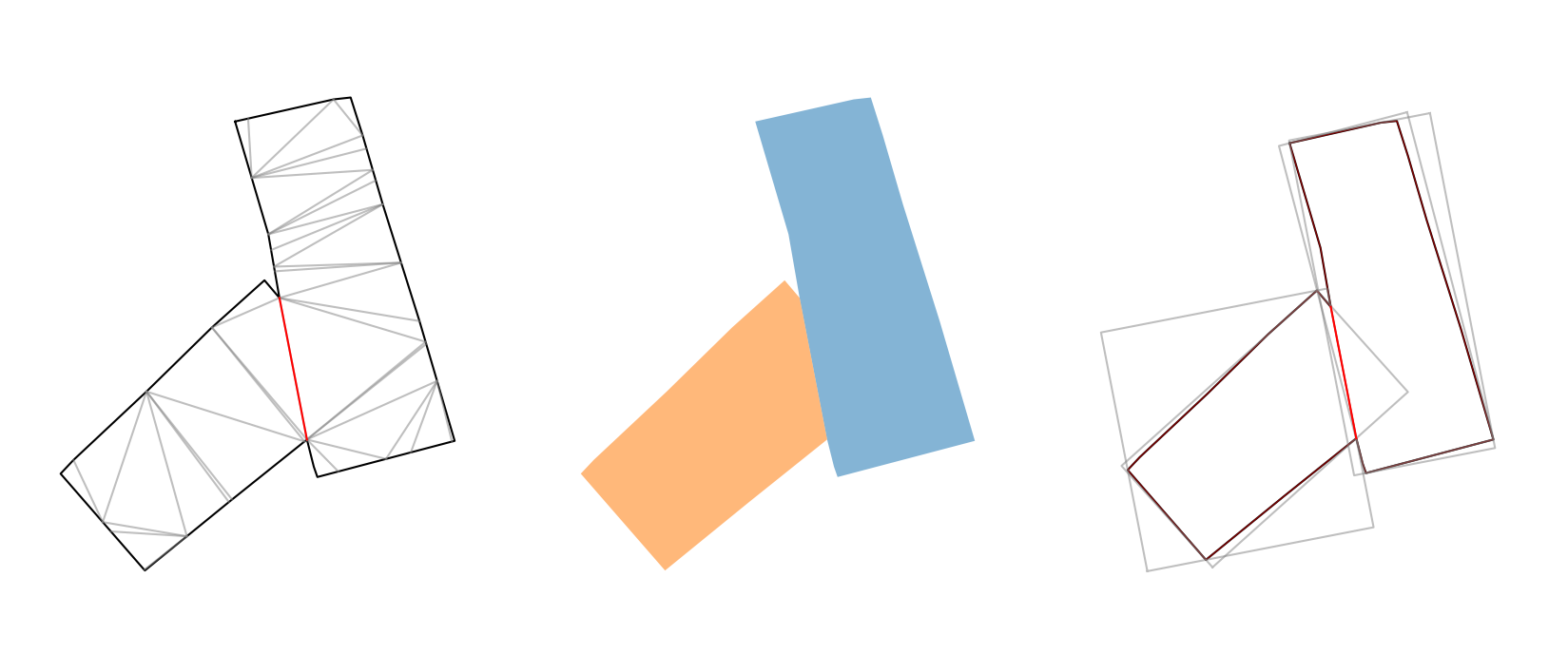
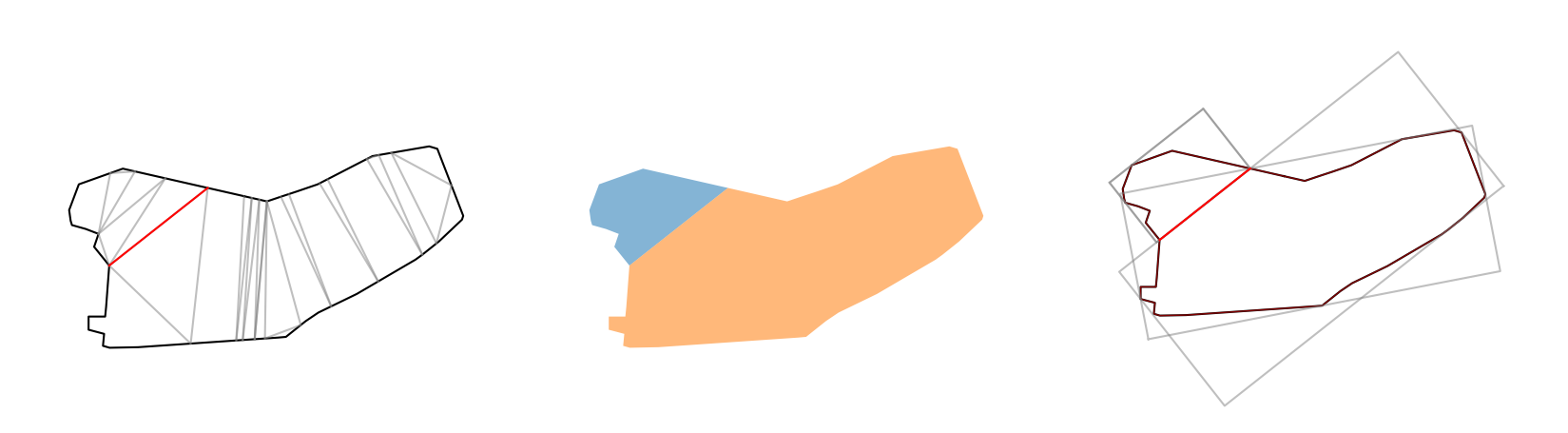
하지만 이 알고리즘은 완벽하지 않으며, 몇 가지 문제가 있습니다. 이 알고리즘은 점수 계산에 weight를 사용하기 때문에 이에 민감할 수 있습니다. 아래 그림들을 보면, 좋은 예시와 나쁜 예시를 각가 보실 수 있습니다. Results of the algorithm From the left, triangulations · segmentations · oriented bounding boxes for segmentations
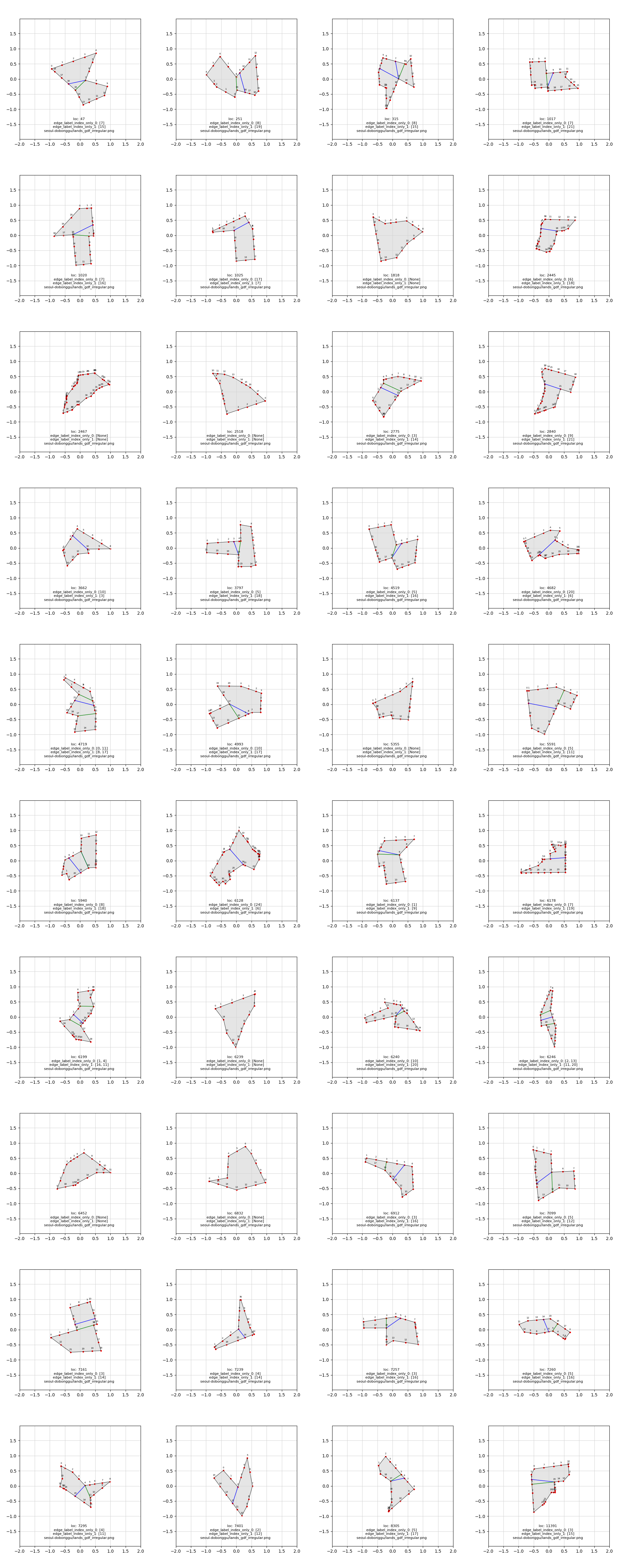
이러한 문제들은 위에서 소개한 알고리즘으로 처리할 수 없기 때문에, 먼저 알고리즘을 사용하여 원시 다각형 데이터를 처리한 다음 다음과 같이 수동으로 라벨링했습니다. 이제 증강된 원본을 포함하여 약 40000개의 데이터를 보유하고 있습니다. 전체 데이터셋은 여기에서 확인할 수 있습니다. Some data for training
Model for link prediction
이제 Pytorch Geometric을 사용하여 graph 모델을 만들고 graph 데이터를 학습시켜 보겠습니다. Pytorch Geometric은 PyTorch를 기반으로 graph neural network를 쉽게 작성하고 학습할 수 있게 해주는 라이브러리입니다.
모델에 부여해야 할 역할은 다각형을 분할할 선들을 생성하는 것입니다. 이는 GNN에서 주로 사용되는 link prediction이라는 작업으로 해석될 수 있습니다. Link prediction 모델은 일반적으로 encoder-decoder 구조를 사용합니다. Encoder는 노드의 특성을 추출하는 벡터 표현인 node embedding을 생성합니다. Decoder는 이러한 embedding을 사용하여 노드 쌍이 연결될 확률을 예측합니다.
추론시에는 모델이 모든 가능한 노드 쌍을 decoder에 입력합니다. 그런 다음 각 쌍이 연결될 확률을 계산합니다. 특정 임계값보다 높은 확률을 가진 쌍만 유지되며, 이는 연결 가능성이 높음을 나타냅니다.
일반적으로 노드 쌍의 유사성을 기반으로 link를 예측하기 위해 내적과 같은 간단한 연산이 사용됩니다. 하지만 저는 이 접근 방식이 geometry 데이터를 사용하는 작업에는 적합하지 않다고 생각하여 decoder를 추가로 학습시켰습니다. 아래는 모델의 encode와 decode 메서드입니다. 전체 모델 코드는 여기에서 확인할 수 있습니다.
    class PolygonSegmenter(nn.Module):
        def __init__(
            self,
            conv_type: str,
            in_channels: int,
            hidden_channels: int,
            out_channels: int,
            encoder_activation: nn.Module,
            decoder_activation: nn.Module,
            predictor_activation: nn.Module,
            use_skip_connection: bool = Configuration.USE_SKIP_CONNECTION,
        ):

            ( ... )

        def encode(self, data: Batch) -> torch.Tensor:
            """Encode the features of polygon graphs

            Args:
                data (Batch): graph batch

            Returns:
                torch.Tensor: Encoded features
            """

            encoded = self.encoder(data.x, data.edge_index, edge_weight=data.edge_weight)

            return encoded

        def decode(self, data: Batch, encoded: torch.Tensor, edge_label_index: torch.Tensor) -> torch.Tensor:
            """Decode the encoded features of the nodes to predict whether the edges are connected

            Args:
                data (Batch): graph batch
                encoded (torch.Tensor): Encoded features
                edge_label_index (torch.Tensor): indices labels

            Returns:
                torch.Tensor: whether the edges are connected
            """

            # Merge raw features and encoded features to inject geometric informations
            if self.use_skip_connection:
                encoded = torch.cat([data.x, encoded], dim=1)

            decoded = self.decoder(torch.cat([encoded[edge_label_index[0]], encoded[edge_label_index[1]]], dim=1)).squeeze()

            return decoded
Encoding 과정은 원본 feature matrix \( F \)를 잠재적으로 다른 차원을 가진 새로운 행렬 \( E \)로 변환합니다. 다음은 encode 함수 전후의 feature matrix 표현입니다.
\( n \)은 노드의 개수
\( m \)은 feature의 개수
\( c \)는 channel의 개수
\( F \in \mathbb{R}^{n \times m} \)는 encode 함수 이전의 feature matrix
\( E \in \mathbb{R}^{n \times c} \)는 encode 함수 이후의 feature matrix
decode 메서드에서는 노드의 encoded feature와 raw feature를 사용하여 노드들 간의 link를 예측합니다. 이 skip connection은 raw feature와 encoded feature를 병합하여 geometry 정보를 주입합니다. Skip connection을 사용하면 원본 특성을 보존하고 low-level과 high-level 정보를 결합하여 전체적인 모델 성능을 향상시킬 수 있습니다.
feedforward 과정에서 decoder는 연결된 레이블과 연결되지 않아야 할 레이블로 학습됩니다. 이는 negative sampling이라고 하는 기법으로, link prediction 작업에서 모델 성능을 향상시키는 데 사용됩니다. 연결되지 않아야 할 예시를 제공함으로써, negative sampling은 모델이 실제 link와 non-link를 더 잘 구분할 수 있게 도와주어 미래 또는 누락된 link를 예측하는 정확도를 향상시킵니다.
대부분의 네트워크에서 실제 link는 non-link보다 훨씬 적기 때문에, 모델이 link가 없다고 예측하는 방향으로 편향될 수 있습니다. Negative sampling은 negative example을 제어된 방식으로 선택할 수 있게 하여 training data의 균형을 맞추고 학습 과정을 향상시킵니다.
        def forward(self, data: Batch) -> Tuple[torch.Tensor, torch.Tensor, torch.Tensor]:
            """Forward method of the models, segmenter and predictor

            Args:
                data (Batch): graph batch

            Returns:
                Tuple[torch.Tensor, torch.Tensor, torch.Tensor]: whether the edges are connected, predicted k and target k
            """

            # Encode the features of polygon graphs
            encoded = self.encode(data)

            ( ... )

            # Sample negative edges
            negative_edge_index = negative_sampling(
                edge_index=data.edge_label_index_only,
                num_nodes=data.num_nodes,
                num_neg_samples=int(data.edge_label_index_only.shape[1] * Configuration.NEGATIVE_SAMPLE_MULTIPLIER),
                method="sparse",
            )

            # Decode the encoded features of the nodes to predict whether the edges are connected
            decoded = self.decode(data, encoded, torch.hstack([data.edge_label_index_only, negative_edge_index]).int())

            return decoded, k_predictions, k_targets
지금까지 encoder와 decoder를 정의했습니다. encoder와 decoder는 batch 단위로 node들을 사용하기 때문에 각각의 graph를 개별적으로 인식할 수 없는 것으로 보입니다. graph가 입력되었을 때 몇 개의 segmentation으로 나눌지를 모델이 학습하기를 원했기 때문에, segmenter 클래스 내에서 k를 별도로 학습하기 위한 predictor를 정의했습니다.
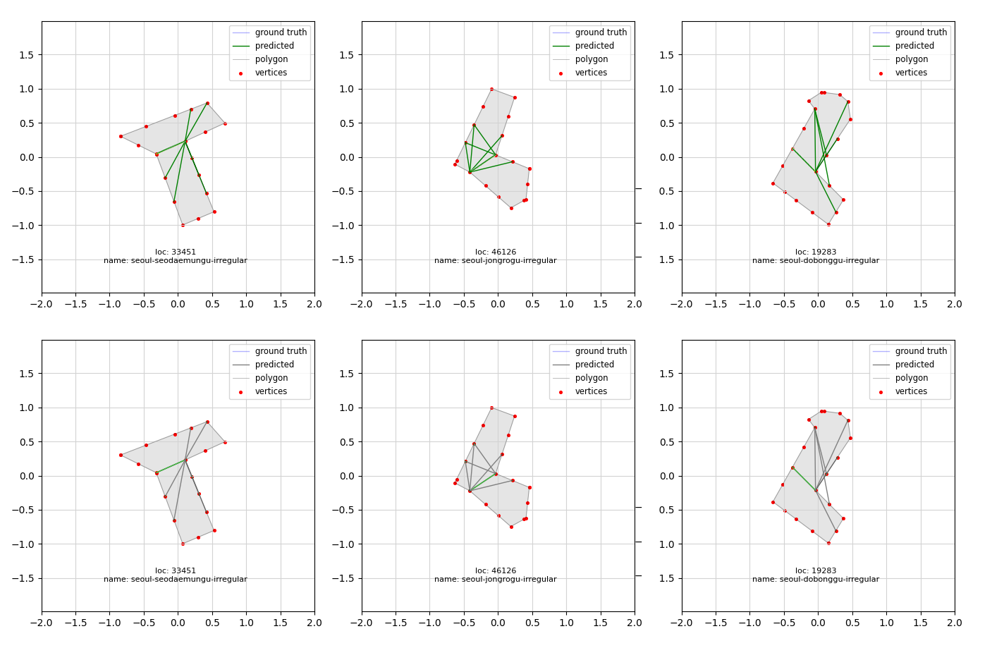
segmenter는 위에서 설명한 encoder와 decoder 과정을 통해 topk를 사용하여 segmentation을 생성합니다. 그런 다음 생성된 link들을 연결 강도 순으로 정렬하고, predictor가 몇 개의 link를 사용할지 결정합니다. Inference process From the top, topk segmentations · segmentation selected by predictor
Training and evaluating
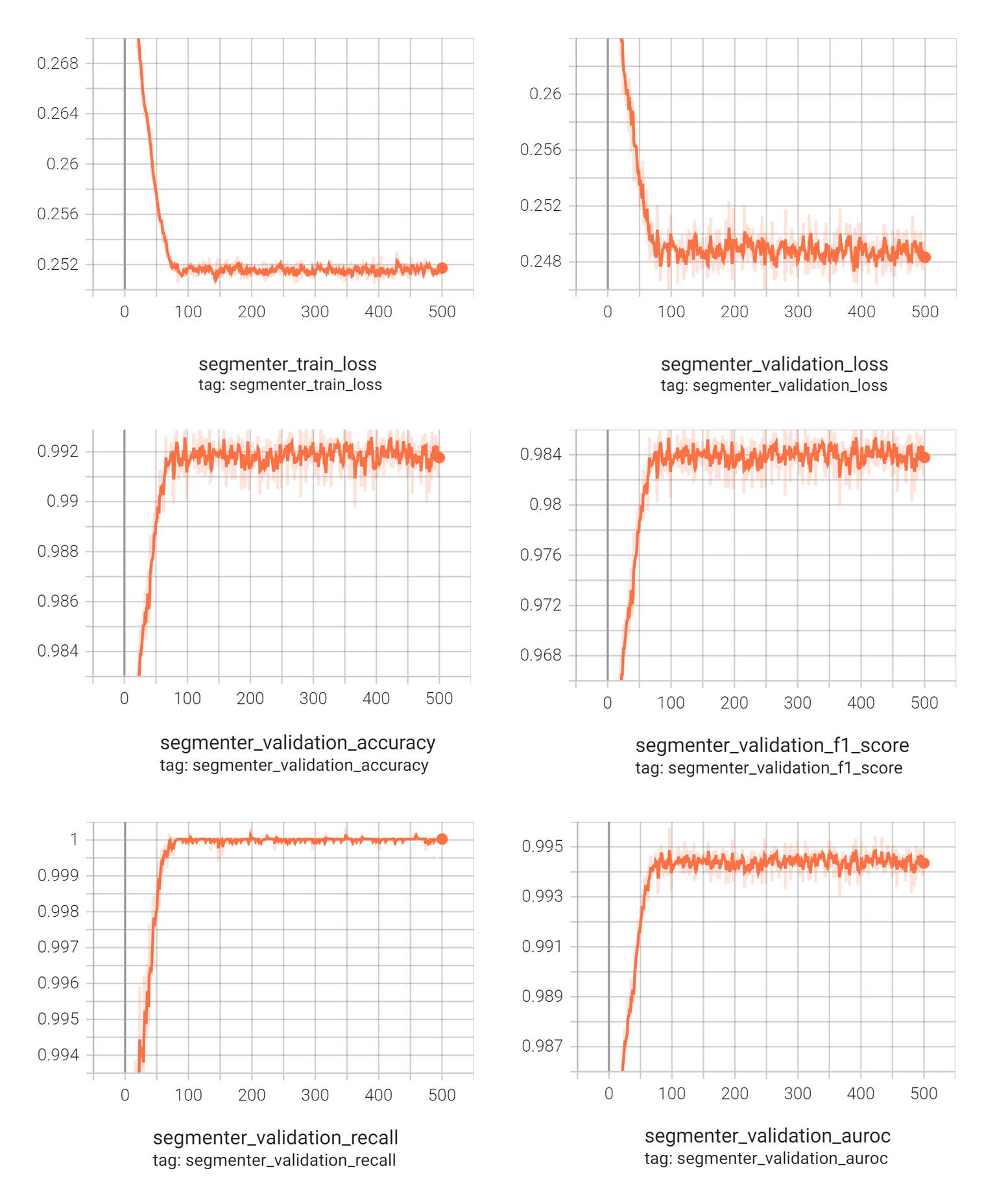
이제 모델을 학습시킬 차례입니다. 모델은 500 epoch 동안 학습되었으며, 이 과정에서 training loss와 validation loss를 기록하여 학습 진행 상황과 수렴도를 모니터링했습니다. 그래프에서 보여지듯이:
상단의 그래프에 따르면, training loss와 validation loss 모두 초기에 빠르게 감소한 다음 일반화됩니다.
모든 평가 지표(accuracy, F1 score, recall, AUROC)가 초기에 빠른 향상을 보인 후 안정화되어 좋은 일반화를 보입니다.
Losses and metrics for 500 epochs
모든 지표가 좋아 보이지만, 이러한 지표들을 100% 신뢰할 수 있는지에 대한 의문이 있습니다. 이는 negative sampling의 영향 때문일 수 있습니다.
일부 test data의 시각화를 기반으로 볼 때, 모델이 분할이 필요하지 않은 다각형을 정확하게 예측한다는 것이 분명합니다. 이는 모델이 negative sample에 대해 overfitting되었을 수 있음을 시사합니다. Negative sample에 대한 높은 성능이 positive case를 정확하게 식별하는 모델의 능력을 정확히 반영하지 못할 수 있습니다. Evaluate some test data qualitatively
IoU loss에서 영감을 받아, segmentation 품질을 평가하고 신뢰할 수 있는 평가 지표를 만들기 위해 GeometricLoss를 정의했습니다. GeometricLoss는 graph 내에서 예측된 geometric 구조와 ground-truth geometric 구조 간의 차이를 정량화하는 것을 목표로 합니다. Geometric loss 계산의 과정은 다음과 같습니다:
Polygon Creation from Node Features: 각 graph의 좌표를 나타내는 node feature들이 다각형으로 변환됩니다.
Connecting Predicted Edges: 이 edge들은 다각형의 예측된 segmentation을 나타냅니다.
Connecting Ground-Truth Edges: 이 edge들은 다각형의 올바른 segmentation을 나타냅니다.
Creating Buffered Unions: 예측된 edge와 ground-truth edge가 결합된 후 buffer 처리됩니다.
Calculating Intersection: 이 교차 영역은 예측된 geometric 구조와 실제 geometric 구조 사이의 공통 영역을 나타냅니다.
Computing Geometric Loss: 교차 영역이 ground-truth 영역으로 정규화된 후 음수화됩니다.
An example for the geometric loss calculation From the left, loss: -0.000478528 · loss: -0.999999994
Geometric loss는 모델의 evaluation metric으로만 사용됩니다. 따라서 BCE loss에 추가되지 않았습니다. 이는 모델의 training batch가 graph가 아닌 node를 기반으로 하기 때문입니다. 따라서 매 epoch마다 모든 graph에 대해 이 loss를 계산하면 처리 속도가 크게 저하될 것입니다. 그래서 batch당 4 sample에 대해서만 이 loss를 계산하여 모델 평가 지표로만 사용했습니다. 결과는 다음과 같습니다. Geometric losses for 500 epochs From the left, train geometric loss · validation geometric loss
GeometricLoss 클래스는 다음과 같이 정의되며 코드는 여기에서 확인할 수 있습니다.
Limitations and future works
GNN은 node embedding 기반 모델이므로 그래프의 기하학적 형상보다는 개별 노드의 특성을 인식하는 것으로 보입니다. GNN은 학습 중에 형태를 일반화하는 능력이 뛰어나지만, 의도한 label에 정확하게 overfit시키는 것은 어려웠습니다.
Comparison with CNNs: CNN은 지역적 패턴을 포착하고 이를 더 추상적인 표현으로 결합하는 데 뛰어나며, 이는 다각형을 다루는 작업에 유리할 수 있습니다.
Imbalanced labels for predictor: predictor는 0, 1, 2 중 하나를 선택하도록 학습되지만, 2에 대한 데이터의 수가 매우 적습니다.
Exploring reliable metrics: geometry 작업에 더 적합한 지표들을 탐색합니다.
Overfitting: positive label을 완전히 overfit할 수 있는 방법을 연구합니다.