Accelerating Reinforcement Batch Inference Speed
Spacewalk is a proptech company that leverages artificial intelligence and data technologies to implement optimal land development scenarios. The architectural design AI, based on reinforcement learning algorithms, creates the most efficient architectural designs. A representative product of the company is Landbook.

Reinforcement learning is a method where an agent, defined within a specific environment, recognizes its current state and selects an action among possible options to maximize rewards. In reinforcement learning using deep learning, the agent learns by performing various actions and receiving rewards accordingly.
To produce high-quality design proposals, it is essential to conduct related research swiftly and efficiently. However, the inference process of architectural design AI has required significant time, necessitating improvements. In this post, we will share a case study on improving the inference time of architectural design AI.
Inference process of architectural AI
The inference process for a single data batch proceeds as follows. In one inference process, the agent and environment interact with each other.
- The agent generates actions based on the current state.
- The environment delivers a new state to the agent based on the agent’s actions.
When these two steps are repeated N times, one inference process is completed.

AS-IS: Using Environment Package
The existing method uses the environment as a Python package. This means that the agent and environment operate on the same computing resources. For environment computations, each operation can be performed independently. Since we typically use computing resources with multiple cores, we process environment operations in parallel according to the number of available cores.
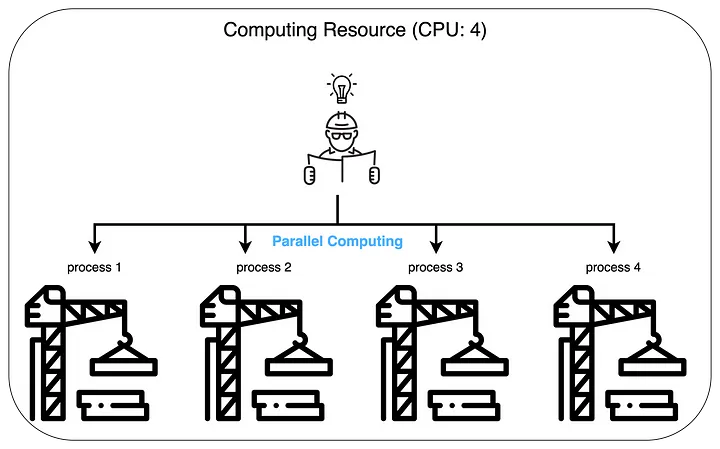
The number of cores in the computing resources used for training directly affects the training speed. For example, let’s compare cases where we have $4$ cores versus $8$ cores when conducting training with a batch size of $128$.
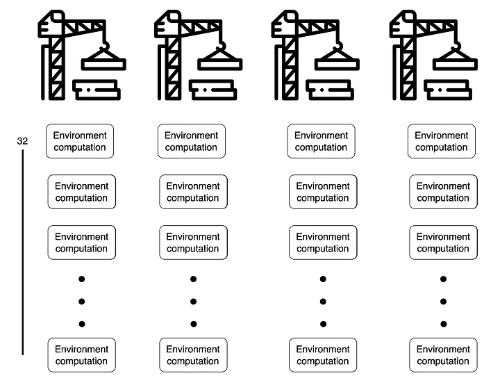
When there are $4$ cores, $128$ environment operations are processed 4 at a time simultaneously. This means that when approximately $128 / 4 = 32$ environment operations are completed on each core, all $128$ environment operations will be finished.
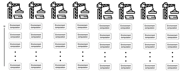
On the other hand, with $8$ cores, $128$ environment operations are processed 8 at a time, meaning that after $128 / 8 = 16$ environment operations, all $128$ operations will be completed. Therefore, compared to the $4$-core case, we can expect the environment computation time to be approximately twice as fast.
However, the number of cores in any given computing resource is physically limited. In other words, cores cannot be increased beyond a certain number. Additionally, the training batch size may increase as models grow larger or research directions change. Therefore, if environment operations are dependent on the computing resources used for training, the training speed will slow down as the batch size increases.
TO-BE: Operating Environment Servers
To make environment computations independent of the agent’s computing resources, we changed the environment from a package form to a server form. This means that the computing resources for agent operations and environment operations can be operated independently.
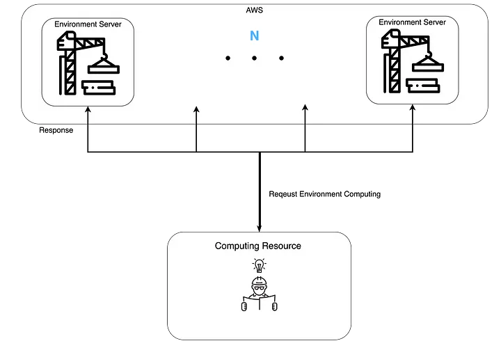
When environment computations are done in server form, there is no limit to the number of simultaneous environment operations that can be processed. Compared to the previous method, the environment server approach can process environment operations simultaneously up to the number of environment servers currently in operation. Additionally, since we use AWS resources, there are no specific limitations on the number of environment servers.
Implementation
Let me introduce how Spacewalk operates the environment servers. Here are the technology stacks we use:
- FastAPI: Framework for implementing environment servers
- AWS: Computing resources needed for environment servers
- Kubernetes: Container orchestration tool for operating environment servers
- Newrelic: Tool for monitoring environment servers
Implementing Environment Servers Using FastAPI
We used the FastAPI framework to implement the environment servers. FastAPI is a Python-based framework with the following advantages. Note that the existing environment package was implemented in Python. For implementation convenience, we built the environment server using Python.
- It’s fast. It shows the best performance among Python frameworks.
- It adopts development standards. OpenAPI (Swagger UI) can be utilized.
- It can be developed with low development costs.
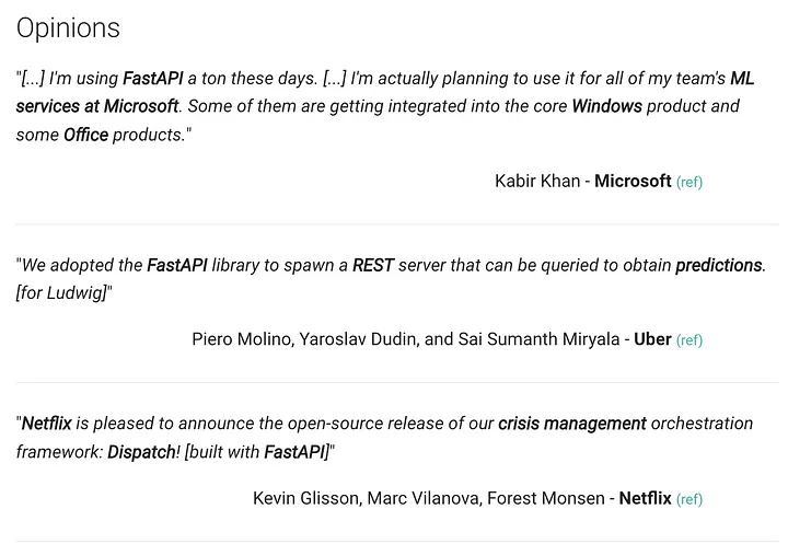
We found that many companies have received quite positive impressions of FastAPI.
The server can be implemented simply with the following code. We implemented it by importing the environment package to use in the environment server.
    from fastapi import FastAPI, File, UploadFile
    import os

    # Environment package
    from swkgym import step
    import pickle
    from fastapi.responses import Response
    from fastapi.logger import logger as fastapi_logger
    import os
    import time
    import sys


    app = FastAPI(
        contact={
            "name": "roundtable",
            "email": "roundtable@spacewalk.tech"
        }
    )


    @app.on_event("startup")
    async def startup_event():
        pass


    @app.post('/step')
    async def step(inputs: UploadFile = File(...),):
        start = time.time()
        bytes = await inputs.read()
        inputs = pickle.loads(bytes)
        fastapi_logger.log(logging.INFO, "Input is Ready")
        # Environment computation
        states = step(inputs["state"], inputs["action"], inputs["p"], inputs["is_training"], inputs["args"])
        fastapi_logger.log(logging.INFO, "Packing Input is Start")
        size_of_response_file = sys.getsizeof(states)
        fastapi_logger.log(logging.INFO, f"response states size is {size_of_response_file} bytes")
        fastapi_logger.log(logging.INFO, f"{inputs['p']} Step time: {time.time() - start}")

        return Response(
            content=pickle.dumps(states)
        )
Using AWS for Dynamic Allocation
As mentioned above, the environment servers use AWS resources. Since architectural AI training is not a constant event (24 hours, every day), purchasing on-premises equipment involves considerable uncertainty. Therefore, we needed to use computing resources dynamically, and we chose AWS, a leading cloud service provider.
Note that AWS’s EKS provides Cluster Autoscaler functionality. This means that as usage increases, the number of nodes (computing resources) that make up the EKS will also increase.
Looking at the actual internal usage patterns of environment servers, we can see the following trends. Since environment servers can be utilized when training architectural design AI, we estimated based on GPU usage rates.
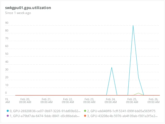
Unlike services that run constantly, requests don’t occur regularly, and when they do occur, the difference compared to when they don’t is quite significant. Therefore, we determined that dynamic resource allocation was reasonable.
Kubernetes(EKS) for Operating Environment Servers
We used Kubernetes to manage environment servers in a stable manner while reducing operational costs. For those interested in learning about Kubernetes, we recommend referring to the official Kubernetes documentation.
Using Kubernetes allows us to systematically handle much of the container management that was previously done manually. For example, instead of having developers manually restart containers when they go down, the system checks container status and automatically recovers them. This is called Self-Healing.
Service discovery and load balancing can also be easily implemented. Environment servers can be exposed externally to allow agent models to access them, and the load on environment servers is distributed using AWS Network Load Balancer.
Additionally, Kubernetes provides Autoscaling functionality. There are two types of Autoscaling: Horizontal Pod Autoscaling and Vertical Pod Autoscaling. Horizontal Pod Autoscaler adjusts the number of Pods with identical resources, while Vertical Pod Autoscaling adjusts the resources allocated to Pods.
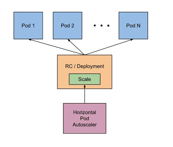
As mentioned earlier, environment server requests do not occur at regular intervals. Therefore, operating the same number of environment servers constantly would be inefficient. We needed to increase the number of environment servers when requests come in and decrease them when there are no requests, which is why we used Kubernetes’ HPA.
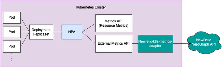
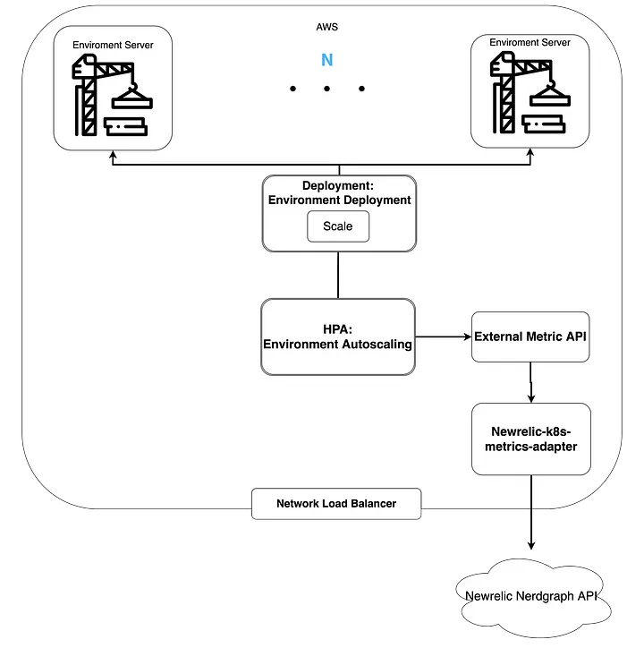
When visualized, the configuration looks like this:
Newrelic Adapter for Defining Environment Server External Metrics
Above, we mentioned using HPA to adjust the number of environment servers. So what criteria can we use to adjust the number of environment servers? At the most basic level, Kubernetes can scale based on pod resource usage:
    type: Resource
    resource:
    name: cpu
    target:
        type: Utilization
        averageUtilization: 60
However, using pod resource usage as an HPA metric for environment servers had some limitations.
In practice, scaling based on CPU usage can lead to the following issues. Let’s assume the average and maximum CPU Utilization for a single request to the environment server is 90%.
- Setting averageUtilization to 90%: The number of Pods doesn’t increase. Even when requests pile up on a single environment server, the number of Pods doesn’t increase. The environment server processes one request at a time, so CPU Utilization remains at an average of 90%.
- Setting averageUtilization below 90%: The number of Pods becomes larger than actually needed. With a batch size of 128, the number of environment servers increases to over 128 to bring averageUtilization below 90%.
For more precise scaling, we needed to know the number of requests per environment server pod. For example, if we set an appropriate request rate of 4 requests per second per environment server pod, we can scale from 1 to 4 environment server pods when 16 requests per second come in.
However, Kubernetes itself doesn’t have the capability to measure request volume for Pods. Instead, we can register custom metrics to use as scaling metrics.
Monitoring tools that can be used with Kubernetes, such as Newrelic or Prometheus, make it easy to register custom metrics. Internally, we use Newrelic to monitor our deployed services. Therefore, we decided to use Newrelic for HPA metrics.
Newrelic is a powerful monitoring tool. And Newrelic provides the New Relic Metrics Adapter. The New Relic Metrics Adapter registers various metrics provided by Newrelic as Kubernetes Metrics.
Installation can be done as follows. Note that if Newrelic is already installed in your Kubernetes Cluster, you can install the New Relic Metrics Adapter separately.
If you meet all of the following requirements, you can easily install it using Helm:
- Kubernetes 1.16 or higher.
- The New Relic Kubernetes integration.
- New Relic’s user API key.
- No other External Metrics should be registered.
    helm upgrade --install newrelic newrelic/nri-bundle \
    --namespace newrelic --create-namespace --reuse-values \
    --set metrics-adapter.enabled=true \
    --set newrelic-k8s-metrics-adapter.personalAPIKey=YOUR_NEW_RELIC_PERSONAL_API_KEY \
    --set newrelic-k8s-metrics-adapter.config.accountID=YOUR_NEW_RELIC_ACCOUNT_ID \
    --set newrelic-k8s-metrics-adapter.config.externalMetrics.{external_metric_name}.query={NRQL query}
Earlier, we mentioned that we needed to scale environment servers based on request volume. For this, we defined the following External Metric:
external_metric_name: env_servier_request_per_secondsNRQL query:
FROM Metric SELECT average(k8s.pod.netRxBytesPerSecond) / {bytes per request} / uniqueCount(k8s.podName) SINCE 1 minute AGO WHERE k8s.deploymentName = 'env-service-deployment'
After installation is complete, you can verify that the External Metric is working properly with the following command:
    $ kubectl get --raw "/apis/external.metrics.k8s.io/v1beta1/namespaces/*/env_servier_request_per_seconds"
    >>> {"kind":"ExternalMetricValueList","apiVersion":"external.metrics.k8s.io/v1beta1","metadata":{},"items":[{"metricName":"env_servier_request_per_seconds","metricLabels":{},"timestamp":"2022-02-08T02:28:17Z","value":"0"}]}
Once we’ve confirmed the metric is working properly, it’s time to deploy the HPA. We can configure the HPA with the following YAML:
    apiVersion: autoscaling/v2beta2
    kind: HorizontalPodAutoscaler
    metadata:
    name: env-service-autoscaling
    spec:
    scaleTargetRef:
        apiVersion: apps/v1
        kind: Deployment
        name: env-service-deployment
    minReplicas: 1
    maxReplicas: 64
    metrics
    - type: External
        external:
        metric:
            name: env_servier_request_per_seconds
            selector:
            matchLabels:
                k8s.namespaceName: default
        target:
            type: Value
            value: "4"
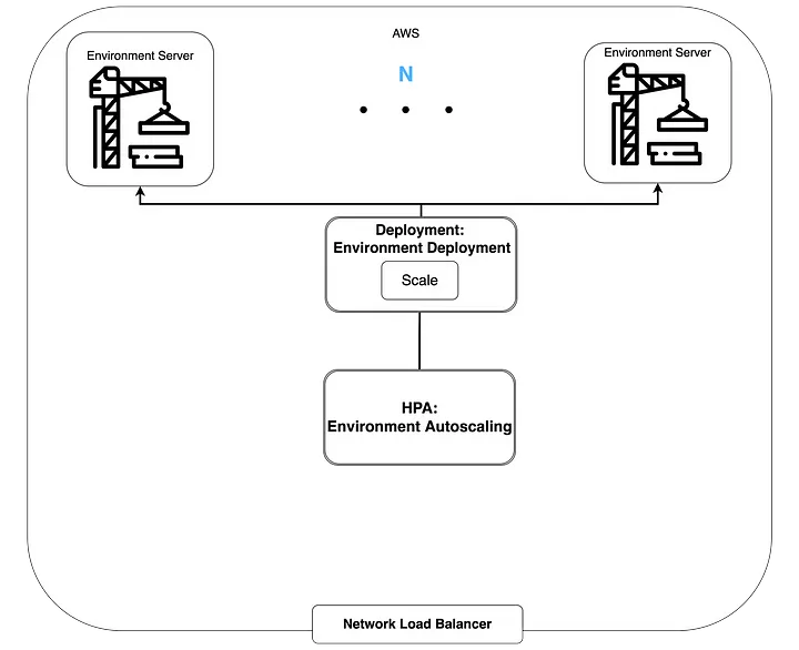
Now that HPA has been fully deployed, the overall diagram looks like this:
Experiments
Let’s examine how much inference speed can be improved when operating environment servers.
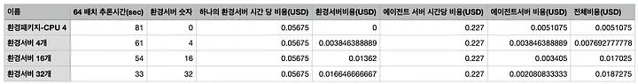
- Agent server: c4.xlarge, $0.227 USD per hour
- Environment server: c4.xlarge/4, $0.061 USD per hour
- AWS cost calculation = (hourly agent server cost + hourly environment server cost * number of servers used) * usage time(seconds) / 3600
- Note that HPA was not applied in the experiments for clear comparison.
There is a difference in inference time between the environment package with 4 CPUs and 4 environment servers. When using CPU inference, the agent model and environment package computations share CPU resources. However, with environment servers, the CPU used by the agent model is separate from the CPU used by the environment package, eliminating processing delays from environmental computations.
In the 64-batch inference experiment, we could reduce the time by about half with triple the AWS costs. We could also reduce the time by about 60% compared to the original with almost similar costs.
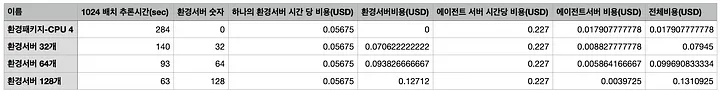
For 1024-batch inference, the parallel processing effect is even more apparent. We could achieve about 4.5 times speed improvement with approximately 7.6 times the cost.
Conclusion
In this post, we covered methods to accelerate batch inference of architectural design AI. When the agent and environment are bound to a single host, the number of cores available for parallel processing is inevitably limited.
To solve this problem, we operated the environment in server form so that the agent and environment could run on independent computing resources. Additionally, since environment server demand is not constant, we utilized cloud services for dynamic computing resources (Cluster Autoscaling) rather than building on-premises resources. We also used Kubernetes’ HPA to automatically adjust the number of environment servers.
We plan to use this batch inference acceleration to improve both the training speed of architectural design AI and service performance.
At Spacewalk, we actively adopt various technology stacks. We will continue to share various internal case studies through future posts.