Floor Plan generation with Voronoi Diagram
11/28/2024, pch-swk
Introduction This project is to review and implement the paper for Free-form Floor Plan Design using Differentiable Voronoi Diagram.
In Deep learning or any gradient-based optimization approach, it uses only tensors to compute gradients, but I think it is not intuitive in geometries. Therefore, I aim to integrate the tensor operations and the geometric operations using Pytorch, Shapely. The biggest difference between the paper and this project is whether using autograd. In the paper, they used the Differentiable Voronoi Diagram for chaining gradient flow, but, I used Numerical Differentiation to approximate the gradients directly. Floor plan generation with voronoi diagram So, what is the numerical differentiation? Numerical Differentiation Numerical differentiation is a method used to approximate a derivative using finite perturbation differences. Unlike automatic differentiation by differentiable voronoi diagram used in the original paper, this approach calculates derivatives by evaluating the function at multiple nearby points. There are three basic methods for numerical differentiation. In this, central difference method is used to compute gradient. Basic methods for the numerical differentiation Central difference method: \[ \begin{align*} \,\\ f'(x) &= \lim_{h \, \rightarrow \, 0} \, \frac{1}{2} \cdot \left( \frac{f(x + h) - f(h)}{h} - \frac{f(x - h) - f(h)}{h} \right) \\\,\\ &= \lim_{h \, \rightarrow \, 0} \, \frac{1}{2} \cdot \frac{f(x + h) - f(x - h)}{h} \\\,\\ &= \lim_{h \, \rightarrow \, 0} \, \frac{f(x + h) - f(x - h)}{2h} \,\\ \end{align*} \] The \(h \,(\text{or } dx)\) in the expression is a perturbation value that determines the accuracy of the approximation. As \(h\) approaches zero, the numerical approximation gets closer to the true derivative. However, in practice, we cannot use an infinitely small value due to computational limitations and floating-point precision. Choosing an appropriate step size is crucial. Too large values lead to poor approximations, while too small values can cause numerical instability due to rounding errors. A stable perturbation value typically ranges from \(h = 10^{-4}\) to \(h = 10^{-6}\). In this implementation, I used \(h = 10^{-6}\) as the perturbation value. Expression of Loss functions In the paper, the key loss functions to optimize floor plans consists of four parts. The below contents are excerpted from the paper: Wall loss: As the unconstrained Voronoi diagram typically produce undesirable fluctuations in the wall orientations, we design a tailored loss function to regularize the wall complexity. Inspired by the Cubic Stylization, we regularize the \(\mathcal{L}_1\) norm of the wall length. \(L_1\) norm is defined as \(v_x + v_y\) (norm of \(x\) + norm of \(y\)), therefore the \(\mathcal{L}_{\text{wall}}\) has the minimal when vector \(\mathbb{v}_j - \mathbb{v}_i\) is vertical or horizontal. \[ \,\\ \mathcal{L}_{\text{wall}} = w_{\text{wall}} \sum_{(v_i, v_j) \, \in \, \mathcal{E}} ||\, \mathbb{v}_i - \mathbb{v}_j \,||_{L1} \,\\ \] where \(\mathcal{E}\) denotes the set of edges of the Voronoi cells between two adjacent rooms and the \(\mathbb{v}_i\) and \(\mathbb{v}_j\) denote the Voronoi vertices belonging to the edge. Area loss: The area of each room is specified by the user. We minimize the quadratic difference between the current room areas and the user-specified targets. Here, \(\bar{A}_r\) denotes the target area for the room \(r\). \[ \,\\ \mathcal{L}_{\text{area}} = w_{\text{area}} \sum_{r=1}^{\#Room} ||\, A_r(\mathcal{V}) - \bar{A}_r \,||^2 \,\\ \] Lloyd loss: To regulate the site density, we design a loss function inspired by the Lloyd's algorithm. Here, \(\mathbb{c}_i \) denotes the centroid of the \(i\)-th Voronoi cell. This is useful for attracting these exterior sites inside \(\Omega\). \[ \,\\ \mathcal{L}_{\text{Lloyd}} = w_{\text{Lloyd}} \sum_{i=1}^N ||\, \mathbb{s}_i - \mathbb{c}_i \,||^2 \,\\ \] Topology loss: We design the topology loss such that each room is a single connected region, and the specified connections between rooms are achieved. We move the site to satisfy the desired topology by setting the goal position \(\mathbb{t}_i\) for each site \(\mathbb{s}_i\) as \[ \,\\ \mathcal{L}_{\text{topo}} = w_{\text{topo}} \sum_{i=1}^N ||\, \mathbb{s}_i - \mathbb{t}_i \,||^2 \,\\ \] The goal position \(\mathbb{t}_i\) can be automatically computed as the nearest site to the site from the same group. For each room, we first group the sites belonging to that room into groups of adjacent sites. If multiple groups are present, that is, a room is split into separated regions, we set the target position of the site \(\mathbb{t}_i\) as the nearest site to that group. Implementation of loss functions As I mentioned in the Introduction, to implement the loss functions above for the forward propagation I used Shapely and Pytorch as below. Total loss is defined as a weighted sum of the above losses, and then using it, the Voronoi diagram generates a floor plan. \[ \,\\ \begin{align*} \mathcal{S}^{*} &= \arg \min_{\mathcal{S}} \mathcal{L}(\mathcal{S}, \mathcal{V}(\mathcal{S})) \\ \mathcal{L} &= \mathcal{L}_{\text{wall}} + \mathcal{L}_{\text{area}} + \mathcal{L}_{\text{fix}} + \mathcal{L}_{\text{topo}} + \mathcal{L}_{\text{Lloyd}} \end{align*} \,\\ \] class FloorPlanLoss(torch. autograd. Function): @staticmethod def compute_wall_loss(rooms_group: List[List[geometry. Polygon]], w_wall: float = 1. 0): loss_wall = 0. 0 for room_group in rooms_group: room_union = ops. unary_union(room_group) if isinstance(room_union, geometry. MultiPolygon): room_union = list(room_union. geoms) else: room_union = [room_union] for room in room_union: t1 = torch. tensor(room. exterior. coords[:-1]) t2 = torch. roll(t1, shifts=-1, dims=0) loss_wall += torch. abs(t1 - t2). sum(). item() for interior in room. interiors: t1 = torch. tensor(interior. coords[:-1]) t2 = torch. roll(t1, shifts=-1, dims=0) loss_wall += torch. abs(t1 - t2). sum(). item() loss_wall = torch. tensor(loss_wall) loss_wall *= w_wall return loss_wall @staticmethod def compute_area_loss( cells: List[geometry. Polygon], target_areas: List[float], room_indices: List[int], w_area: float = 1. 0, ): current_areas = [0. 0] * len(target_areas) for cell, room_index in zip(cells, room_indices): current_areas[room_index] += cell. area current_areas = torch. tensor(current_areas) target_areas = torch. tensor(target_areas) area_difference = torch. abs(current_areas - target_areas) loss_area = torch. sum(area_difference) loss_area **= 2 loss_area *= w_area return loss_area @staticmethod def compute_lloyd_loss(cells: List[geometry. Polygon], sites: torch. Tensor, w_lloyd: float = 1. 0): valids = [(site. tolist(), cell) for site, cell in zip(sites, cells) if not cell. is_empty] valid_centroids = torch. tensor([cell. centroid. coords[0] for _, cell in valids]) valid_sites = torch. tensor([site for site, _ in valids]) loss_lloyd = torch. norm(valid_centroids - valid_sites, dim=1). sum() loss_lloyd **= 2 loss_lloyd *= w_lloyd return loss_lloyd @staticmethod def compute_topology_loss(rooms_group: List[List[geometry. Polygon]], w_topo: float = 1. 0): loss_topo = 0. 0 for room_group in rooms_group: room_union = ops. unary_union(room_group) if isinstance(room_union, geometry. MultiPolygon): largest_room, *_ = sorted(room_union. geoms, key=lambda r: r. area, reverse=True) loss_topo += len(room_union. geoms) for room in room_group: if not room. intersects(largest_room) and not room. is_empty: loss_topo += largest_room. centroid. distance(room) loss_topo = torch. tensor(loss_topo) loss_topo **= 2 loss_topo *= w_topo return loss_topo ( . . . ) @staticmethod def forward( ctx: FunctionCtx, sites: torch. Tensor, boundary_polygon: geometry. Polygon, target_areas: List[float], room_indices: List[int], w_wall: float, w_area: float, w_lloyd: float, w_topo: float, w_bb: float, w_cell: float, save: bool = True, ) -> torch. Tensor: cells = [] walls = [] sites_multipoint = geometry. MultiPoint([tuple(point) for point in sites. detach(). numpy()]) raw_cells = list(shapely. voronoi_polygons(sites_multipoint, extend_to=boundary_polygon). geoms) for cell in raw_cells: intersected_cell = cell. intersection(boundary_polygon) intersected_cell_iter = [intersected_cell] if isinstance(intersected_cell, geometry. MultiPolygon): intersected_cell_iter = list(intersected_cell. geoms) for intersected_cell in intersected_cell_iter: exterior_coords = torch. tensor(intersected_cell. exterior. coords[:-1]) exterior_coords_shifted = torch. roll(exterior_coords, shifts=-1, dims=0) walls. extend((exterior_coords - exterior_coords_shifted). tolist()) cells. append(intersected_cell) cells_sorted = [] raw_cells_sorted = [] for site_point in sites_multipoint. geoms: for ci, (cell, raw_cell) in enumerate(zip(cells, raw_cells)): if raw_cell. contains(site_point): cells_sorted. append(cell) cells. pop(ci) raw_cells_sorted. append(raw_cell) raw_cells. pop(ci) break rooms_group = [[] for _ in torch. tensor(room_indices). unique()] for cell, room_index in zip(cells_sorted, room_indices): rooms_group[room_index]. append(cell) loss_wall = torch. tensor(0. 0) if w_wall > 0: loss_wall = FloorPlanLoss. compute_wall_loss(rooms_group, w_wall=w_wall) loss_area = torch. tensor(0. 0) if w_area > 0: loss_area = FloorPlanLoss. compute_area_loss(cells_sorted, target_areas, room_indices, w_area=w_area) loss_lloyd = torch. tensor(0. 0) if w_lloyd > 0: loss_lloyd = FloorPlanLoss. compute_lloyd_loss(cells_sorted, sites, w_lloyd=w_lloyd) loss_topo = torch. tensor(0. 0) if w_topo > 0: loss_topo = FloorPlanLoss. compute_topology_loss(rooms_group, w_topo=w_topo) loss_bb = torch. tensor(0. 0) if w_bb > 0: loss_bb = FloorPlanLoss. compute_bb_loss(rooms_group, w_bb=w_bb) loss_cell_area = torch. tensor(0. 0) if w_cell > 0: loss_cell_area = FloorPlanLoss. compute_cell_area_loss(cells_sorted, w_cell=w_cell) if save: ctx. save_for_backward(sites) ctx. room_indices = room_indices ctx. target_areas = target_areas ctx. boundary_polygon = boundary_polygon ctx. w_wall = w_wall ctx. w_area = w_area ctx. w_lloyd = w_lloyd ctx. w_topo = w_topo ctx. w_bb = w_bb ctx. w_cell = w_cell loss = loss_wall + loss_area + loss_lloyd + loss_topo + loss_bb + loss_cell_area return loss, [loss_wall, loss_area, loss_lloyd, loss_topo, loss_bb, loss_cell_area] Since I tried to intuitively convert the loss functions to Python codes with Shapely, there are some differences compared to the original. Backward with numerical differentiation Using numerical differentiation is not efficient in terms of computational performance. This is because it requires multiple function evaluations at nearby points to approximate derivatives. As you can see in the backward method, computational performance is influenced by the number of given sites. Therefore, I used Python's built-in multiprocessing module to improve the performance of backward propagation. @staticmethod def _backward_one(args): ( sites, i, j, epsilon, boundary_polygon, target_areas, room_indices, w_wall, w_area, w_lloyd, w_topo, w_bb, w_cell, ) = args perturbed_sites_pos = sites. clone() perturbed_sites_neg = sites. clone() perturbed_sites_pos[i, j] += epsilon perturbed_sites_neg[i, j] -= epsilon loss_pos, _ = FloorPlanLoss. forward( None, perturbed_sites_pos, boundary_polygon, target_areas, room_indices, w_wall, w_area, w_lloyd, w_topo, w_bb, w_cell, save=False, ) loss_neg, _ = FloorPlanLoss. forward( None, perturbed_sites_neg, boundary_polygon, target_areas, room_indices, w_wall, w_area, w_lloyd, w_topo, w_bb, w_cell, save=False, ) return i, j, (loss_pos - loss_neg) / (2 * epsilon) @runtime_calculator @staticmethod def backward(ctx: FunctionCtx, _: torch. Tensor, __): sites = ctx. saved_tensors[0] room_indices = ctx. room_indices target_areas = ctx. target_areas boundary_polygon = ctx. boundary_polygon w_wall = ctx. w_wall w_area = ctx. w_area w_lloyd = ctx. w_lloyd w_topo = ctx. w_topo w_bb = ctx. w_bb w_cell = ctx. w_cell epsilon = 1e-6 grads = torch. zeros_like(sites) multiprocessing_args = [ ( sites, i, j, epsilon, boundary_polygon, target_areas, room_indices, w_wall, w_area, w_lloyd, w_topo, w_bb, w_cell, ) for i in range(sites. size(0)) for j in range(sites. size(1)) ] with multiprocessing. Pool(processes=multiprocessing. cpu_count()) as pool: results = pool. map(FloorPlanLoss. _backward_one, multiprocessing_args) for i, j, grad in results: grads[i, j] = grad return grads, None, None, None, None, None, None, None, None, None, None Initializing parameters In optimization problems, the initial parameters significantly affect the final results. Firstly, I initialized the Voronoi diagram's sites such that the sites were generated at the center of a given floor plan: Random Sites Generation: Generate initial random sites using uniform distribution. Moving to Center of Boundary: Shift all sites so they are centered within the floor plan boundary. Outside Sites Adjustment: Adjust any sites that fall outside the boundary by moving them inward. Voronoi Diagram: Generate Voronoi diagram using sites. Process of parameters initialization Secondly, I used the KMeans clustering algorithm to assign cell indices per each site. Distance-based KMeans algorithm groups sites based on their spatial proximity, which helps ensure that rooms are formed from adjacent cells. By pre-clustering the sites, I created initial room assignments that are already spatially coherent, reducing the possibility of disconnected room regions during optimization. Using this approach, the optimizer converges more stably. Let me give an example: Floor plan generation on 300 iterations From the left, optimization without KMeans · optimization with KMeans As you can see in the figure above, KMeans makes the loss flow more smoothly and converge faster. Without KMeans, the optimization process shows erratic behavior with disconnected rooms. In contrast, when using KMeans for initial room assignments, the optimization maintains spatial coherence throughout the process, leading to: Faster convergence to the target room areas More stable wall alignments Reduced possibility of rooms splitting into disconnected regions This improvement in optimization stability is particularly important for complex floor plans with multiple rooms and specific area requirements. Experiments Finally, I'll conclude this article by attaching the experimental results optimized by 800 iterations. The boundaries for experiments are used in the original paper and repository. Please refer to this project repository for the entire code. Future works Set entrance: In the paper, to set entrance of the plan it uses \(\mathcal{L}_{\text{fix}}\) loss function. Graph-based contraint: In the paper, to set and ensure the rooms' adjacencies it uses graph-based constraint. Improve computational performance: Optimize the code to run faster (converting used language, or implementing differentiable voronoi diagram). Handle deadspaces: Set the loss function for deadspace \(\mathcal{L}_{\text{deadspace}}\) to exclude infeasible plans. Following boundary axis: Align walls to follow the axis of a given boundary instead of global X, Y (Replacing \(\mathcal{L}_{\text{wall}}\)). . .