Floor Plan generation with Voronoi Diagram
11/28/2024, pch-swk
Introduction 본 프로젝트는 논문 리뷰 및 Free-form Floor Plan Design using Differentiable Voronoi Diagram 논문을 구현하는 것입니다. 딥러닝이나 경사하강법 기반의 최적화 접근법에서는 그래디언트를 계산하기 위해 텐서만을 사용하지만, 이는 기하학적으로 직관적이지 않습니다 따라서 이 프로젝트에서는 Pytorch와 Shapely를 사용하여 텐서 연산과 기하학적 연산을 통합합니다.
본 논문과 이 프로젝트의 가장 큰 차이점은 autograd의 사용 여부입니다. 논문에서는 그래디언트 흐름을 연결하기 위해 Differentiable Voronoi Diagram을 사용했지만, 여기서는 그래디언트를 직접 근사하기 위해 수치 미분 (Numerical Differentiation) 방식을 채택했습니다. Floor plan generation with voronoi diagram 먼저 수치 미분 (Numerical Differentiation)에 대해서 알아보겠습니다. Numerical Differentiation 수치 미분 (Numerical differentiation)은 finite perturbation differences를 사용하여 도함수를 근사하는 방법입니다. 원 논문에서 사용된 미분 가능한 보로노이 다이어그램을 통한 자동 미분과 달리, 이 방식은 여러 인접한 지점에서 함수를 평가하여 도함수를 계산합니다. 수치 미분에는 세 가지 기본적인 방법이 있습니다. 이 프로젝트에서는 그래디언트를 계산하기 위해 중앙 차분법을 사용했습니다. Basic methods for the numerical differentiation Central difference method: \[ \begin{align*} \,\\ f'(x) &= \lim_{h \, \rightarrow \, 0} \, \frac{1}{2} \cdot \left( \frac{f(x + h) - f(h)}{h} - \frac{f(x - h) - f(h)}{h} \right) \\\,\\ &= \lim_{h \, \rightarrow \, 0} \, \frac{1}{2} \cdot \frac{f(x + h) - f(x - h)}{h} \\\,\\ &= \lim_{h \, \rightarrow \, 0} \, \frac{f(x + h) - f(x - h)}{2h} \,\\ \end{align*} \] 수식에서 \(h \,(\text{또는 } dx)\)는 근사의 정확도를 결정하는 perturbation differences 값입니다. \(h\)가 0에 가까워질수록 수치적 근사는 실제 도함수에 더 가까워집니다. 하지만 실제로는 계산상의 한계와 부동소수점 정밀도 때문에 무한히 작은 값을 사용할 수 없습니다. 적절한 스텝 크기를 선택하는 것이 중요합니다. 너무 큰 값은 부정확한 근사를 초래하고, 반대로 너무 작은 값은 반올림 오차로 인한 수치적 불안정성을 야기할 수 있습니다. 안정적인 섭동값은 일반적으로 \(h = 10^{-4}\)에서 \(h = 10^{-6}\) 사이의 범위를 가집니다. 이 구현에서는 섭동값으로 \(h = 10^{-6}\)을 사용했습니다. Expression of Loss functions 원 논문에서 최적화에 사용되는 주요 손실 함수는 네 가지 부분으로 구성됩니다. 아래 내용은 논문에서 발췌된 내용입니다: Wall loss: Unconstrained Voronoi diagram 은 일반적으로 벽면 방향에 원치 않는 변동을 만들어내기 때문에, 벽면의 복잡도를 제어하기 위한 맞춤형 손실 함수를 설계했습니다. Cubic Stylization에서 영감을 받아, 벽면 길이의 \(\mathcal{L}_1\) 노름을 정규화했습니다. \(L_1\) 노름은 \(v_x + v_y\) (x의 노름 + y의 노름)로 정의되며, 따라서 벡터 \(\mathbb{v}_j - \mathbb{v}_i\)가 수직 또는 수평일 때 \(\mathcal{L}_{\text{wall}}\)이 최소값을 가집니다. \[ \,\\ \mathcal{L}_{\text{wall}} = w_{\text{wall}} \sum_{(v_i, v_j) \, \in \, \mathcal{E}} ||\, \mathbb{v}_i - \mathbb{v}_j \,||_{L1} \,\\ \] 여기서 \(\mathcal{E}\)는 인접한 두 방 사이의 보로노이 셀 경계선 집합을 나타내며, \(\mathbb{v}_i\)와 \(\mathbb{v}_j\)는 해당 경계선에 속한 보로노이 꼭짓점들을 나타냅니다. Area loss: 각 방의 면적은 사용자가 지정합니다. 현재 방 면적과 사용자가 지정한 목표 면적 간의 제곱 차이를 최소화합니다. 여기서 \(\bar{A}_r\)은 방 \(r\)의 목표 면적을 나타냅니다. \[ \,\\ \mathcal{L}_{\text{area}} = w_{\text{area}} \sum_{r=1}^{\#Room} ||\, A_r(\mathcal{V}) - \bar{A}_r \,||^2 \,\\ \] Lloyd loss: 사이트 밀도를 조절하기 위해 Lloyd's algorithm에서 영감을 받은 손실 함수를 설계했습니다. 여기서 \(\mathbb{c}_i\)는 \(i\)번째 보로노이 셀의 중심점을 나타냅니다. 이는 외부 사이트들을 \(\Omega\) 내부로 끌어들이는 데 유용합니다. \[ \,\\ \mathcal{L}_{\text{Lloyd}} = w_{\text{Lloyd}} \sum_{i=1}^N ||\, \mathbb{s}_i - \mathbb{c}_i \,||^2 \,\\ \] Topology loss: 각 방이 하나의 연결된 영역이 되도록 하고, 방들 간의 지정된 연결이 이루어지도록 위상 손실을 설계했습니다. 각 사이트 \(\mathbb{s}_i\)에 대한 목표 위치 \(\mathbb{t}_i\)를 설정하여 원하는 위상을 만족하도록 사이트를 이동시킵니다. \[ \,\\ \mathcal{L}_{\text{topo}} = w_{\text{topo}} \sum_{i=1}^N ||\, \mathbb{s}_i - \mathbb{t}_i \,||^2 \,\\ \] 목표 위치 \(\mathbb{t}_i\)는 같은 그룹 내에서 가장 가까운 사이트로 자동 계산됩니다. 각 방에 대해, 먼저 해당 방에 속한 사이트들을 인접한 사이트들의 그룹으로 묶습니다. 만약 여러 그룹이 존재한다면, 즉 방이 분리된 영역들로 나뉘어 있다면, 해당 그룹에서 가장 가까운 사이트를 사이트 \(\mathbb{t}_i\)의 목표 위치로 설정합니다. Implementation of loss functions 서론에서 언급했듯이, 순전파를 위한 위의 손실 함수들을 구현하기 위해 아래와 같이 Shapely와 Pytorch를 사용했습니다. 전체 손실은 위에서 설명한 손실들의 가중합으로 정의되며, 이를 사용하여 보로노이 다이어그램이 평면도를 생성합니다. \[ \,\\ \begin{align*} \mathcal{S}^{*} &= \arg \min_{\mathcal{S}} \mathcal{L}(\mathcal{S}, \mathcal{V}(\mathcal{S})) \\ \mathcal{L} &= \mathcal{L}_{\text{wall}} + \mathcal{L}_{\text{area}} + \mathcal{L}_{\text{fix}} + \mathcal{L}_{\text{topo}} + \mathcal{L}_{\text{Lloyd}} \end{align*} \,\\ \] class FloorPlanLoss(torch. autograd. Function): @staticmethod def compute_wall_loss(rooms_group: List[List[geometry. Polygon]], w_wall: float = 1. 0): loss_wall = 0. 0 for room_group in rooms_group: room_union = ops. unary_union(room_group) if isinstance(room_union, geometry. MultiPolygon): room_union = list(room_union. geoms) else: room_union = [room_union] for room in room_union: t1 = torch. tensor(room. exterior. coords[:-1]) t2 = torch. roll(t1, shifts=-1, dims=0) loss_wall += torch. abs(t1 - t2). sum(). item() for interior in room. interiors: t1 = torch. tensor(interior. coords[:-1]) t2 = torch. roll(t1, shifts=-1, dims=0) loss_wall += torch. abs(t1 - t2). sum(). item() loss_wall = torch. tensor(loss_wall) loss_wall *= w_wall return loss_wall @staticmethod def compute_area_loss( cells: List[geometry. Polygon], target_areas: List[float], room_indices: List[int], w_area: float = 1. 0, ): current_areas = [0. 0] * len(target_areas) for cell, room_index in zip(cells, room_indices): current_areas[room_index] += cell. area current_areas = torch. tensor(current_areas) target_areas = torch. tensor(target_areas) area_difference = torch. abs(current_areas - target_areas) loss_area = torch. sum(area_difference) loss_area **= 2 loss_area *= w_area return loss_area @staticmethod def compute_lloyd_loss(cells: List[geometry. Polygon], sites: torch. Tensor, w_lloyd: float = 1. 0): valids = [(site. tolist(), cell) for site, cell in zip(sites, cells) if not cell. is_empty] valid_centroids = torch. tensor([cell. centroid. coords[0] for _, cell in valids]) valid_sites = torch. tensor([site for site, _ in valids]) loss_lloyd = torch. norm(valid_centroids - valid_sites, dim=1). sum() loss_lloyd **= 2 loss_lloyd *= w_lloyd return loss_lloyd @staticmethod def compute_topology_loss(rooms_group: List[List[geometry. Polygon]], w_topo: float = 1. 0): loss_topo = 0. 0 for room_group in rooms_group: room_union = ops. unary_union(room_group) if isinstance(room_union, geometry. MultiPolygon): largest_room, *_ = sorted(room_union. geoms, key=lambda r: r. area, reverse=True) loss_topo += len(room_union. geoms) for room in room_group: if not room. intersects(largest_room) and not room. is_empty: loss_topo += largest_room. centroid. distance(room) loss_topo = torch. tensor(loss_topo) loss_topo **= 2 loss_topo *= w_topo return loss_topo ( . . . ) @staticmethod def forward( ctx: FunctionCtx, sites: torch. Tensor, boundary_polygon: geometry. Polygon, target_areas: List[float], room_indices: List[int], w_wall: float, w_area: float, w_lloyd: float, w_topo: float, w_bb: float, w_cell: float, save: bool = True, ) -> torch. Tensor: cells = [] walls = [] sites_multipoint = geometry. MultiPoint([tuple(point) for point in sites. detach(). numpy()]) raw_cells = list(shapely. voronoi_polygons(sites_multipoint, extend_to=boundary_polygon). geoms) for cell in raw_cells: intersected_cell = cell. intersection(boundary_polygon) intersected_cell_iter = [intersected_cell] if isinstance(intersected_cell, geometry. MultiPolygon): intersected_cell_iter = list(intersected_cell. geoms) for intersected_cell in intersected_cell_iter: exterior_coords = torch. tensor(intersected_cell. exterior. coords[:-1]) exterior_coords_shifted = torch. roll(exterior_coords, shifts=-1, dims=0) walls. extend((exterior_coords - exterior_coords_shifted). tolist()) cells. append(intersected_cell) cells_sorted = [] raw_cells_sorted = [] for site_point in sites_multipoint. geoms: for ci, (cell, raw_cell) in enumerate(zip(cells, raw_cells)): if raw_cell. contains(site_point): cells_sorted. append(cell) cells. pop(ci) raw_cells_sorted. append(raw_cell) raw_cells. pop(ci) break rooms_group = [[] for _ in torch. tensor(room_indices). unique()] for cell, room_index in zip(cells_sorted, room_indices): rooms_group[room_index]. append(cell) loss_wall = torch. tensor(0. 0) if w_wall > 0: loss_wall = FloorPlanLoss. compute_wall_loss(rooms_group, w_wall=w_wall) loss_area = torch. tensor(0. 0) if w_area > 0: loss_area = FloorPlanLoss. compute_area_loss(cells_sorted, target_areas, room_indices, w_area=w_area) loss_lloyd = torch. tensor(0. 0) if w_lloyd > 0: loss_lloyd = FloorPlanLoss. compute_lloyd_loss(cells_sorted, sites, w_lloyd=w_lloyd) loss_topo = torch. tensor(0. 0) if w_topo > 0: loss_topo = FloorPlanLoss. compute_topology_loss(rooms_group, w_topo=w_topo) loss_bb = torch. tensor(0. 0) if w_bb > 0: loss_bb = FloorPlanLoss. compute_bb_loss(rooms_group, w_bb=w_bb) loss_cell_area = torch. tensor(0. 0) if w_cell > 0: loss_cell_area = FloorPlanLoss. compute_cell_area_loss(cells_sorted, w_cell=w_cell) if save: ctx. save_for_backward(sites) ctx. room_indices = room_indices ctx. target_areas = target_areas ctx. boundary_polygon = boundary_polygon ctx. w_wall = w_wall ctx. w_area = w_area ctx. w_lloyd = w_lloyd ctx. w_topo = w_topo ctx. w_bb = w_bb ctx. w_cell = w_cell loss = loss_wall + loss_area + loss_lloyd + loss_topo + loss_bb + loss_cell_area return loss, [loss_wall, loss_area, loss_lloyd, loss_topo, loss_bb, loss_cell_area] 손실 함수들을 Shapely를 이용해 직관적인 파이썬 코드로 구현하는 과정에서, 원본 논문과는 다소 차이가 있습니다. Backward with numerical differentiation 수치 미분은 계산 성능 측면에서 효율적이지 않습니다. 이는 도함수를 근사하기 위해 여러 인접 지점에서 함수를 반복적으로 계산해야 하기 때문입니다. backward 메서드에서 볼 수 있듯이, 계산 성능은 주어진 사이트의 개수에 따라 크게 영향을 받습니다. 따라서 역전파 성능을 개선하기 위해 파이썬의 내장 멀티프로세싱 모듈을 사용했습니다. @staticmethod def _backward_one(args): ( sites, i, j, epsilon, boundary_polygon, target_areas, room_indices, w_wall, w_area, w_lloyd, w_topo, w_bb, w_cell, ) = args perturbed_sites_pos = sites. clone() perturbed_sites_neg = sites. clone() perturbed_sites_pos[i, j] += epsilon perturbed_sites_neg[i, j] -= epsilon loss_pos, _ = FloorPlanLoss. forward( None, perturbed_sites_pos, boundary_polygon, target_areas, room_indices, w_wall, w_area, w_lloyd, w_topo, w_bb, w_cell, save=False, ) loss_neg, _ = FloorPlanLoss. forward( None, perturbed_sites_neg, boundary_polygon, target_areas, room_indices, w_wall, w_area, w_lloyd, w_topo, w_bb, w_cell, save=False, ) return i, j, (loss_pos - loss_neg) / (2 * epsilon) @runtime_calculator @staticmethod def backward(ctx: FunctionCtx, _: torch. Tensor, __): sites = ctx. saved_tensors[0] room_indices = ctx. room_indices target_areas = ctx. target_areas boundary_polygon = ctx. boundary_polygon w_wall = ctx. w_wall w_area = ctx. w_area w_lloyd = ctx. w_lloyd w_topo = ctx. w_topo w_bb = ctx. w_bb w_cell = ctx. w_cell epsilon = 1e-6 grads = torch. zeros_like(sites) multiprocessing_args = [ ( sites, i, j, epsilon, boundary_polygon, target_areas, room_indices, w_wall, w_area, w_lloyd, w_topo, w_bb, w_cell, ) for i in range(sites. size(0)) for j in range(sites. size(1)) ] with multiprocessing. Pool(processes=multiprocessing. cpu_count()) as pool: results = pool. map(FloorPlanLoss. _backward_one, multiprocessing_args) for i, j, grad in results: grads[i, j] = grad return grads, None, None, None, None, None, None, None, None, None, None Initializing parameters 최적화 문제에서는 초기 매개변수가 최종 결과에 큰 영향을 미칩니다. 먼저, 보로노이 다이어그램의 사이트들이 주어진 평면도의 중심에 생성되도록 초기화했습니다: Random Sites Generation: 균일 분포를 사용하여 초기 무작위 사이트들을 생성합니다. Moving to Center of Boundary: 모든 사이트를 평면도 경계의 중심으로 이동시킵니다. Outside Sites Adjustment: 경계 밖으로 벗어난 사이트들을 안쪽으로 이동시켜 조정합니다. Voronoi Diagram: 사이트들을 사용하여 보로노이 다이어그램을 생성합니다. Process of parameters initialization 두 번째로, 각 사이트별 셀 인덱스를 할당하기 위해 KMeans 클러스터링 알고리즘을 사용했습니다. 거리 기반 KMeans 알고리즘은 사이트들의 공간적 근접성을 기준으로 그룹화하며, 이는 인접한 셀들로부터 방이 형성되도록 보장하는 데 도움이 됩니다. 사이트들을 사전에 클러스터링함으로써, 이미 공간적으로 연결된 초기 방 배치를 생성할 수 있었고, 이는 최적화 과정에서 방이 분리된 영역으로 나뉠 가능성을 줄여줍니다. 이러한 접근 방식을 사용하면 최적화가 더 안정적으로 수렴합니다. 예시를 보여드리겠습니다: Floor plan generation on 300 iterations From the left, optimization without KMeans · optimization with KMeans 위 그림에서 볼 수 있듯이, KMeans를 사용하면 손실이 더 부드럽게 흐르고 더 빠르게 수렴합니다. KMeans를 사용하지 않으면, 최적화 과정에서 방들이 분리되는 불안정한 동작을 보입니다. 반면에, 초기 방 할당에 KMeans를 사용하면 최적화 과정 전반에 걸쳐 공간적 일관성이 유지되어 다음과 같은 장점이 있습니다: 목표 방 면적으로 더 빠른 수렴 더 안정적인 벽체 정렬 방이 분리된 영역으로 나뉠 가능성 감소 이러한 최적화 안정성의 향상은 특히 여러 개의 방과 특정 면적 요구사항이 있는 복잡한 평면도에서 중요합니다. Experiments 마지막으로, 800회 반복으로 최적화된 실험 결과들을 첨부하며 이 글을 마무리하겠습니다. 실험에 사용된 경계들은 원 논문과 저장소에서 가져왔습니다. 전체 코드는 이 프로젝트의 저장소를 참고해 주시기 바랍니다. Future works Set entrance: 논문에서는 평면도의 출입구를 설정하기 위해 \(\mathcal{L}_{\text{fix}}\) 손실 함수 사용. Graph-based contraint: 논문에서는 방들 간의 인접성을 설정하고 보장하기 위해 그래프 기반 제약을 사용. Improve computational performance: 코드 실행 속도 최적화 (사용 언어 변경 또는 미분 가능한 보로노이 다이어그램 구현). Handle deadspaces: 실현 불가능한 평면도를 제외하기 위해 Deadspace에 대한 손실 함수 \(\mathcal{L}_{\text{deadspace}}\) 설정. Following boundary axis: 전역 X, Y축 대신 주어진 경계의 축을 따라 벽면 정렬 (\(\mathcal{L}_{\text{wall}}\) 대체). . .