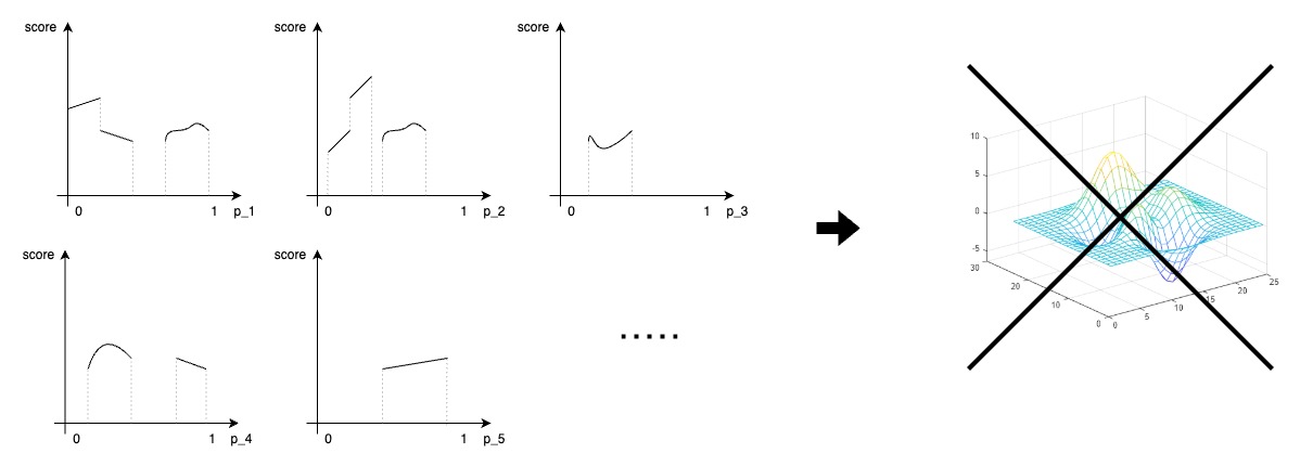
Finding Differentiable Environments
Abstract
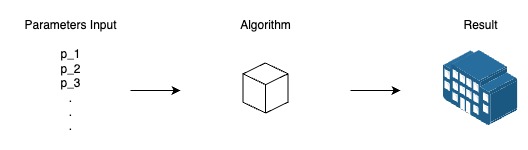
- When implementing architectural algorithms or parametric design, it’s easy to think of them as algorithms that produce results based on parameters.
- However, in heuristic optimizers like GA or ES, the algorithm itself becomes an environment that changes parameters,
- Furthermore, when used as a criterion for model learning, and in the case of reinforcement learning, the environment becomes the standard itself for judging the model’s directionality.
- As part of exploring what characteristics the environment should have, we investigated the significance of differentiable environments and tested the results.
- We set up two environments: one with definite gradient cutoff and another without it,
- And by comparing gradient descent, AdamW, and GA methods, we were able to confirm the significance of differentiable environments.
Problem
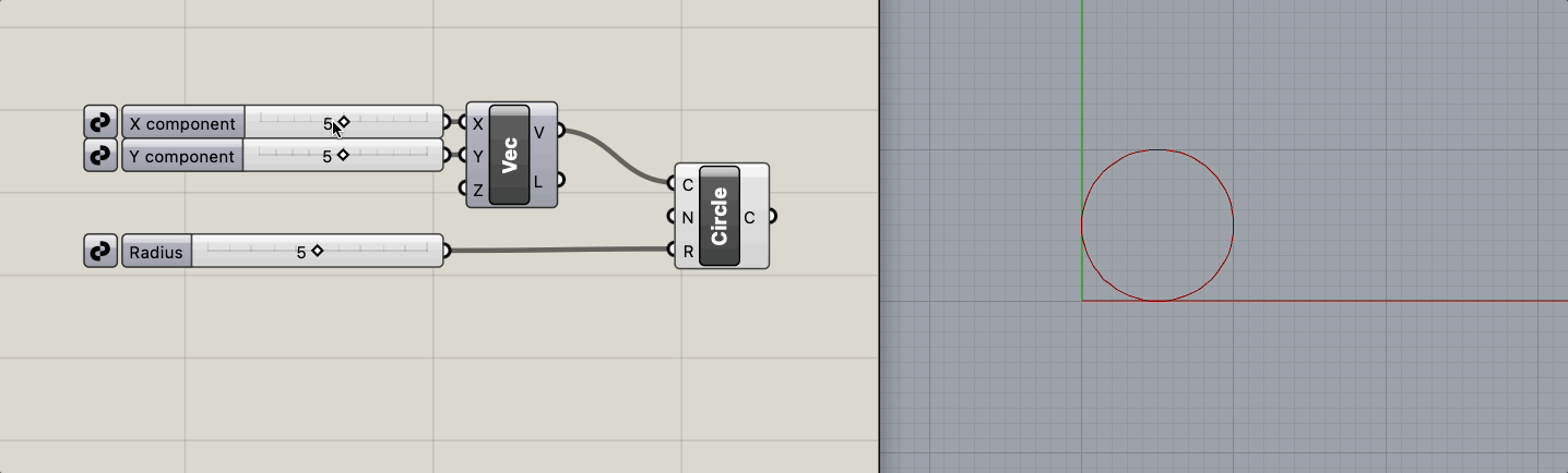
Creating an environment for architectural algorithms - or parametric design environments - intuitively takes the following form:
    Generate a circle with position and radius as parameters.
    Loss is defined as one-tenth of the difference between the circle's area and the area of a circle with radius 5 (25).
When the logic is simple like this, there’s usually not much disconnect between parameters and results.
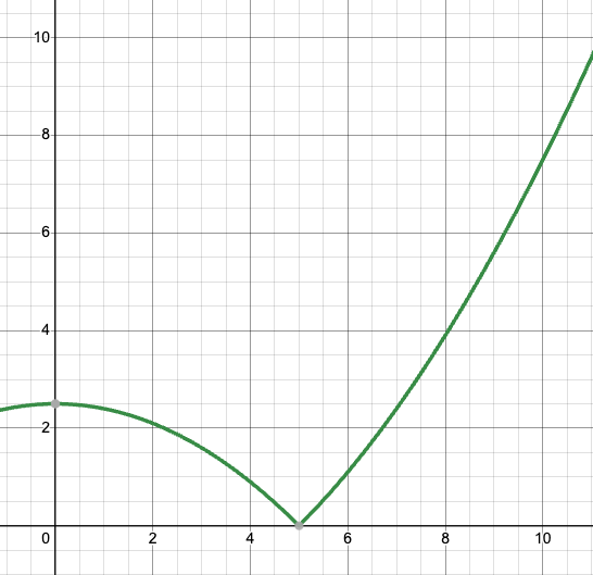
The radius-loss graph can be expressed as follows (for x >= 0):
However, as algorithms become more complex, this environment becomes a black box,
and even the developers find it difficult to understand the tendencies of results based on parameters.
This is where the problem arises.
- Even without considering reinforcement learning models, optimization processes like GA also need to “measure” results based on parameter changes.
- However, the randomness of parameter differences’ impact on the environment is too high, making the results based on parameter changes excessively random.
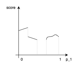
The above figure shows the problem even with just one parameter. However, in architectural algorithm engines, it’s almost impossible to use just one or two parameters. This means that not only smooth curves showing tendencies are difficult to identify, but optimization modules can hardly grasp the tendencies.
 There will be no continuous engine without continuous [parameter - loss].
 Therefore, we started by consciously trying to make the score (or negative loss) that the environment creates with parameters and their corresponding environment differentiable when adding any environment functions and parameters.
Premises
- Including parametric design algorithms, the environment mentioned in this post refers to a module that can calculate geometry-related data and loss from input parameters.
- To explicitly ensure differentiability or parameter connectivity, all processes from starting parameters to loss calculation are performed only through torch tensor operations.
Environment Details
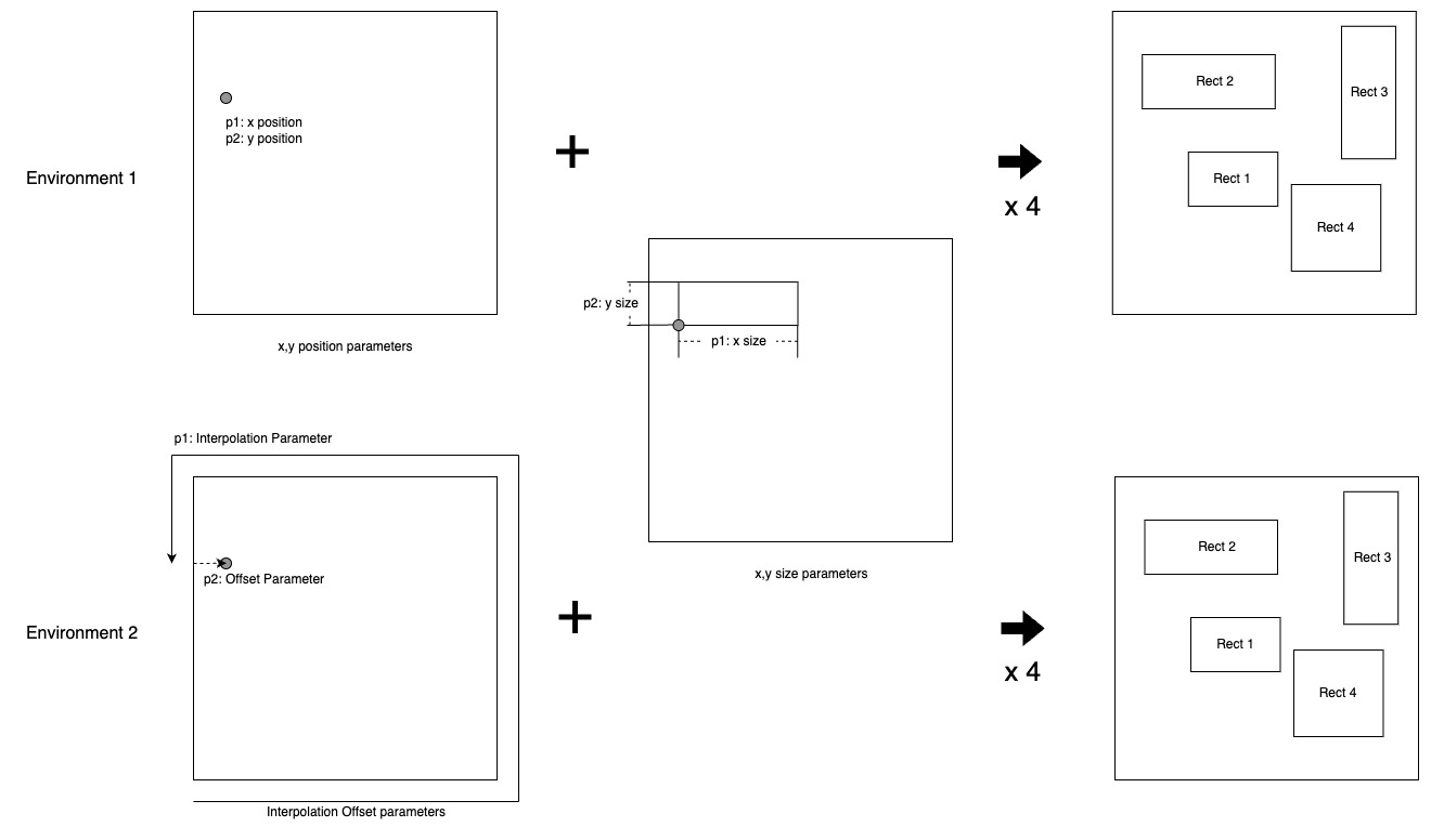
1. Parameter and Loss Definition for Environment
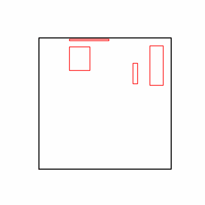
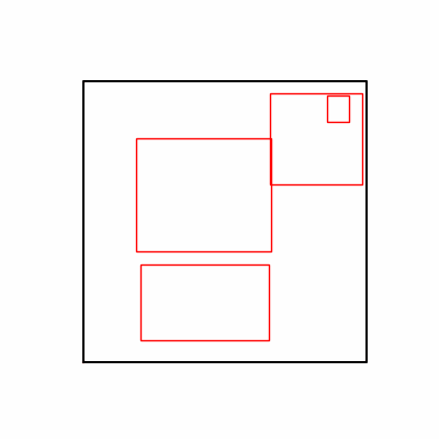
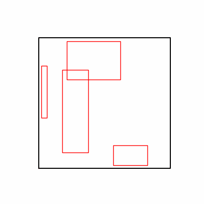
- Parameter Definition - Total 16 parameters
- Environment 1 - x, y position ratio for 4 rectangles
- (x_ratio, y_ratio) corresponds to each rectangle’s width and height, ensuring one-to-one correspondence with (x, y) position.
- (x_ratio, y_ratio) corresponds to each rectangle’s width and height, ensuring one-to-one correspondence with (x, y) position.
- Environment 2 - interpolation, offset ratio for 4 rectangles
- offset operates based on 0.5 of the corresponding width or height, ensuring one-to-one correspondence with (x, y) position generated through this.
- In other words, there is definite gradient cutoff.
- Environment 1 - x, y position ratio for 4 rectangles
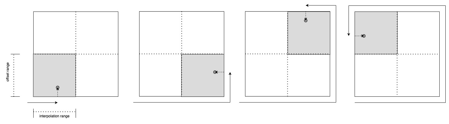 Using 0.5 for dividing 4 quadrants in Environment 2
- Common - x, y size ratio for 4 rectangles - After position is determined, x_size and y_size are determined through ratio from remaining possible distance.
- In other words, both environments look at the same search space where for every point (x, y) ∈ ℝ² in 2D plane, there exists a one-to-one corresponding parameter to generate it.
- Loss Definition (Each loss is multiplied by a coefficient and added to the final loss)
- L1: Variance of each rectangle’s area (to make each rectangle have similar areas)
$$ \displaystyle L1 = \frac{1}{n} \sum_{i=1}^{n} (Area(Rectangle_i) - \mu)^2 $$- L2: Sum of overlapping areas between rectangles (to prevent rectangles from overlapping)
$$ \displaystyle L2 = \sum_{i=1}^{n} \sum_{j=i+1}^{n} Area(Rectangle_i \cap Rectangle_j) $$- L3: Aspect ratio of each rectangle (deviation from 1.5)
$$ \displaystyle L3 = \sum_{i=1}^{n} \left| \frac{\max(w_i, h_i)}{\min(w_i, h_i)} - 1.5 \right| $$- L4: Sum of areas of all rectangles (area should be large)
$$ \displaystyle L4 = \sum_{i=1}^{n} Area(Rectangle_i) $$
Checking Differentiability through Primitive Gradient Descent
    # This is not an optimizer that modifies the learning model's weights,
    # but rather differentiable programming that directly updates the parameters used for generating results.
    optimizer = torch.optim.SGD([parameters], lr=learning_rate)
- sigmoid was used to keep parameters in 0 ~ 1 range.
- We tested both environments using a simple method of reflecting backpropagated gradients to parameters.
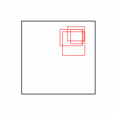
- Environment 1 showed more consistent tendencies, had smaller final loss values, and produced actual shape arrangements closer to the intended results.
- (However, since the Loss is not complete but rather for understanding test tendencies, we’ll focus more on the Loss numbers themselves rather than the actual shape arrangement images.)
- (However, since the Loss is not complete but rather for understanding test tendencies, we’ll focus more on the Loss numbers themselves rather than the actual shape arrangement images.)
- In other words, while both environments look at the same search space, Environment 1 can be considered more differentiable.
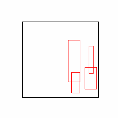
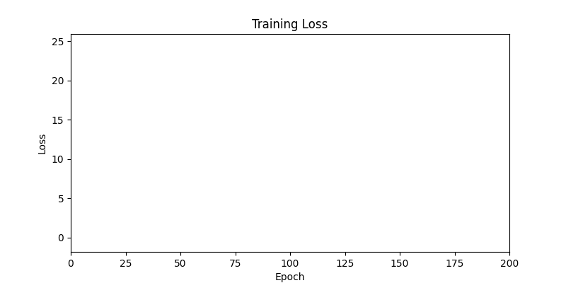
- Environment 1

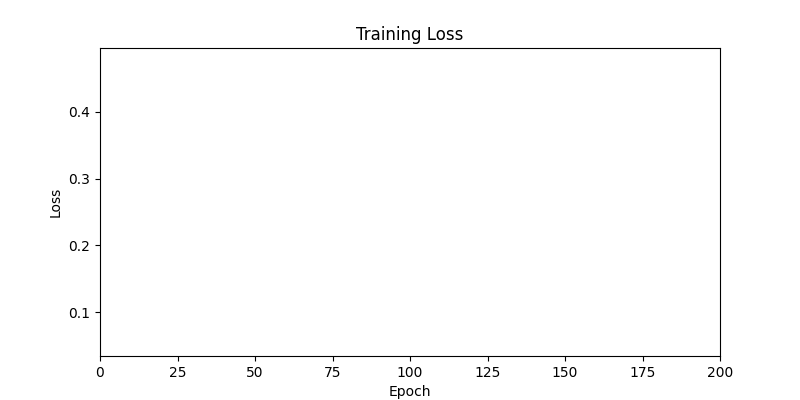
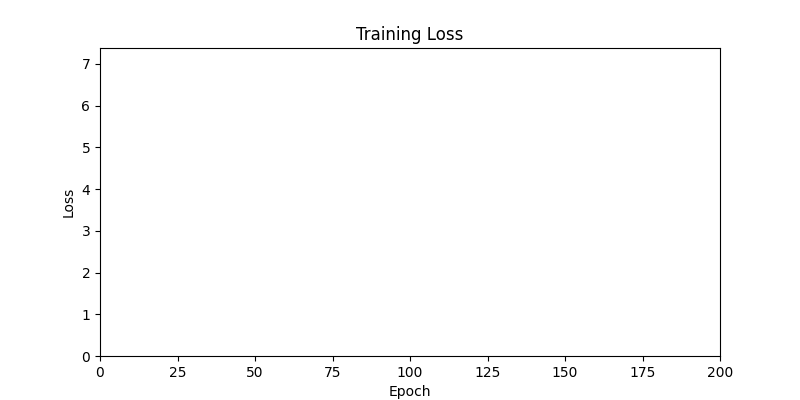
- Environment 2


- Now we’ll proceed with optimization using GA module and Adam optimizer with these two environments.
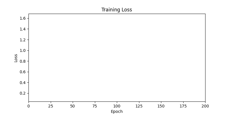
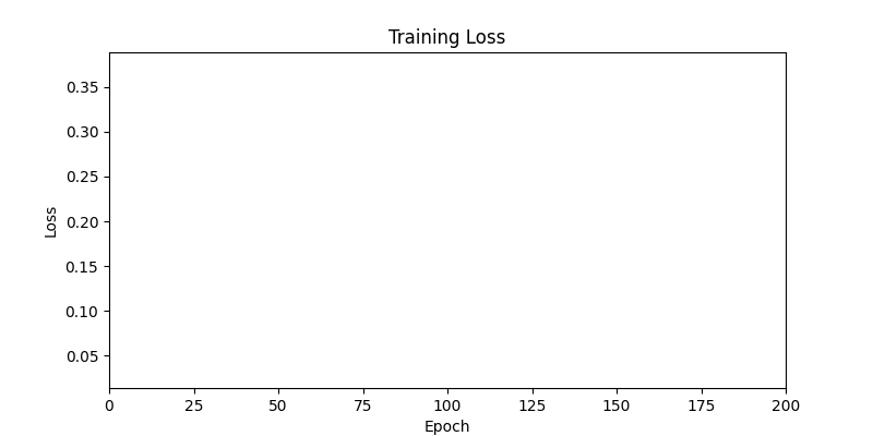
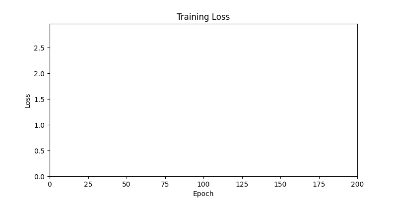
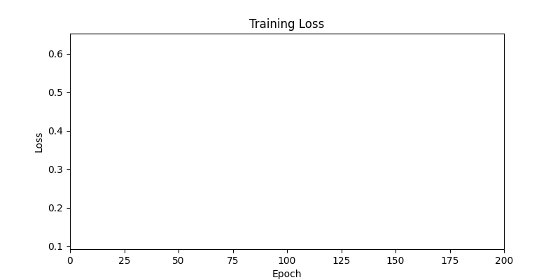
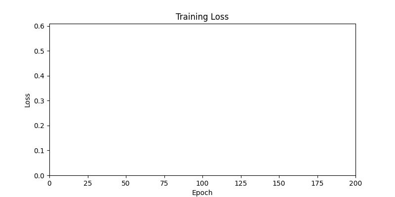
1. Optimization Test Results using AdamW Optimizer
optimizer = torch.optim.AdamW([parameters], lr=learning_rate)
- Environment 1

- Environment 2
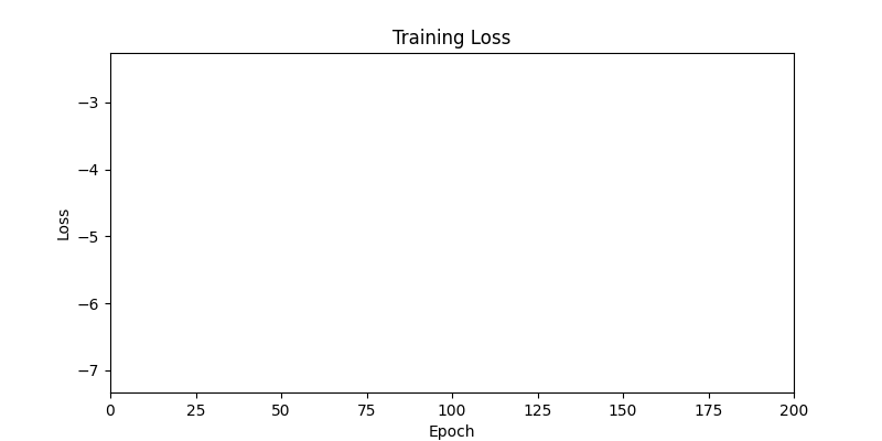
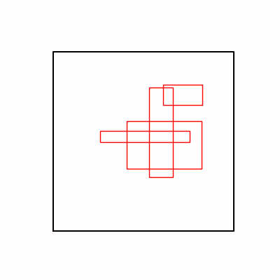
2. Optimization Test Results using Genetic Algorithm
- In GA, the final results are similar. With sufficient computation, since the search space itself is the same, we can confirm that they converge to almost identical scores.
- However, it’s often impossible to provide sufficient computation every time. Moving quickly towards the answer is also important. We can confirm that Environment 1 definitely has better initial stability.
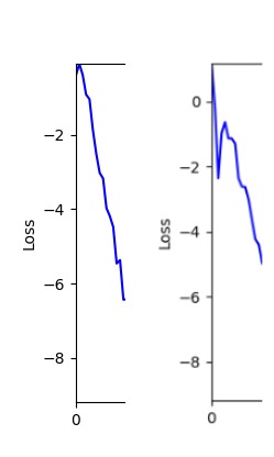 Difference in initial graphs between two environments
 - Moreover, in GA we used a Population of 100 per generation. In other words, this is the result of performing 20,000 computations, unlike the previous two cases which only performed 200 computations. While using GA might be one way to guarantee final performance, it’s difficult to consider it an efficient method at least among these three. (Only 200 computations in 2 generations)
- Environment 1


- Environment 2


Conclusion
- We confirmed that differentiable environments, where changes in parameters lead to continuous changes in the environment or results, can achieve better results in the optimization process.
- This tendency was observed not only in simple gradient descent or AdamW, but even in optimization algorithms like GA.
- While it may not be possible to apply this to all parameters, we reaffirmed that it’s meaningful to consciously try to add parameters in a differentiable form to the environment when possible during development.
-
- To achieve similar scores, GA required many more execution counts. This suggests there might be more efficient methods than GA. We expect to be able to reduce the total number of computations through differentiable environments and methods or other approaches.
- To achieve similar scores, GA required many more execution counts. This suggests there might be more efficient methods than GA. We expect to be able to reduce the total number of computations through differentiable environments and methods or other approaches.
- Let’s Use Differentiable Environment!