Latent masses

10/23/2023, pch-swk

Objectives

Generative Adversarial Networks (GANs) have paved the way for unprecedented advancements in numerous areas, from art creation to deepfake video generation. However, the potential of GANs isn't restricted to 2D space. The development and application of 3D GANs have opened new possibilities, especially in the realm of design.

This project delves deep into the possibilities of 3D GANs in the design field with the following objectives:

Grasp the fundamental concepts behind GANs and their 3D extension
Appreciate the power and nuances of 3D GANs through hands-on experiments
Examine how 3D GANs can be harnessed for product design, architectural modeling, and virtual environment creation
visualize and manipulate the latent space to generate novel and innovative designs
Understand the limitations of current 3D GAN models and the potential areas of improvement

By the way, what is GANs(Generative Adversarial Networks)? 🧬

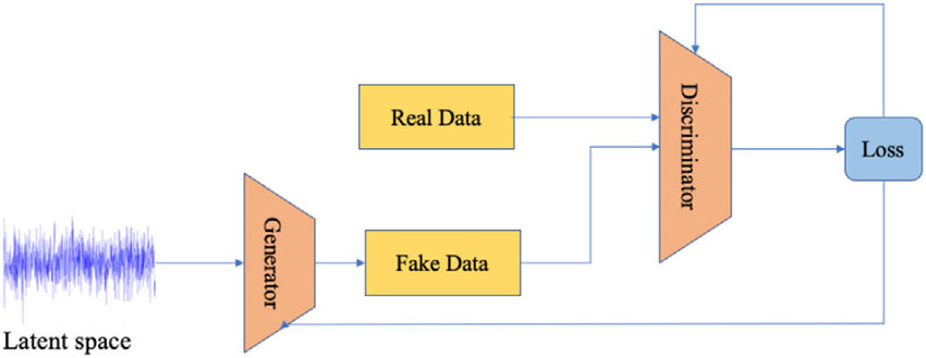
Generative Adversarial Networks, commonly referred to as GANs, are a class of artificial intelligence algorithms designed to generate new data that resemble a given set of data. The architecture of a GAN consists of two primary components:

1. Generator

The role of the generator is to create fake data
It takes in random noise from a latent space and produces data samples as its output
The primary objective of the generator is to produce data that is indistinguishable from real data

2.Discriminator

The discriminator functions as a binary classifier
It aims to differentiate between real and fake data
The discriminator receives both real data samples and the fake data generated by the generator, and its task is to correctly label them as 'real' or 'fake'

The provided diagram illustrates this process, showing how the generator's output is evaluated by the discriminator, resulting in a loss that helps both parts improve.

Generative adversarial networks concept diagram

3D shape representations for the generative adversarial networks

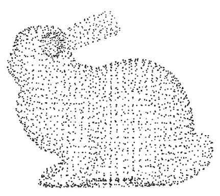
1. Point cloud

A point cloud is a set of data points in space. In 3D shape representation, point clouds are typically used to represent the external surface of an object Each point in the point cloud has an (x, y, z) coordinate
Can represent any 3D shape without being limited to a specific topology or grid (Good at flexibility)
Points are disconnected, so additional processing is often required to extract surfaces or other features (Not good at lack of connectivity)

2. Voxel

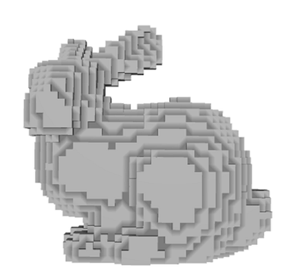
Voxels (short for volumetric pixels) are the 3D equivalent of 2D pixels. A voxel representation divides the 3D space into a regular grid, and each cell (or voxel) in the grid can be either occupied or empty
Operations like convolution are straightforward to apply on voxel grids (Simplicity)
To represent fine details, a very high-resolution grid is needed, which can be computationally prohibitive (Limited resolution)

3. Mesh

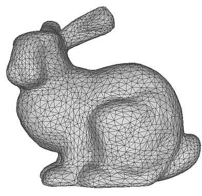
A 3D mesh consists of vertices, edges, and faces that define the shape of a 3D object in space. The most common type of mesh is a triangular mesh, where the shape is represented using triangles
Can represent both simple and complex geometries (Good expressiveness)
Provides information about how points are connected, which is useful for many applications (Good at continuous surface representation)
Operations on meshes, like subdivision or simplification, can be computationally demanding (Complexity)

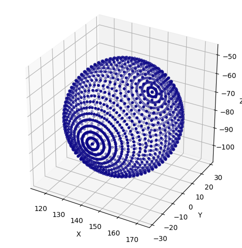
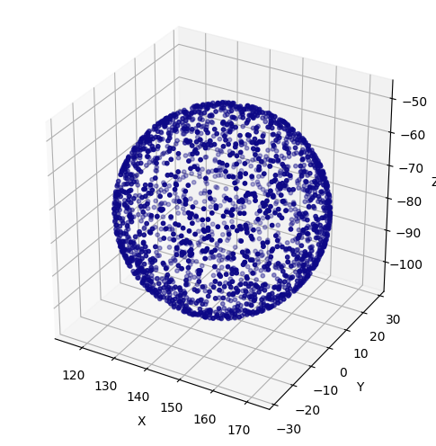
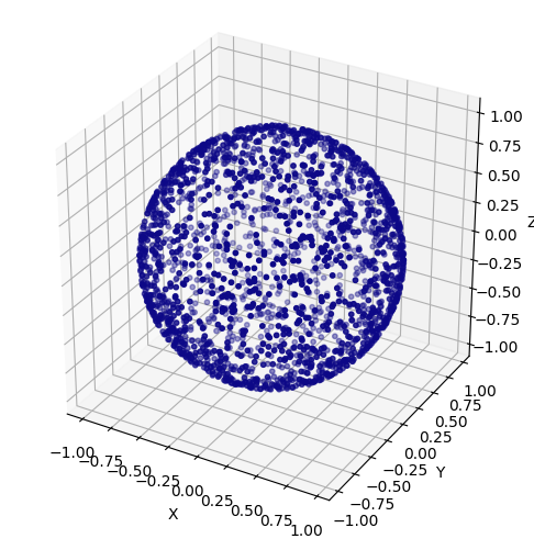
Simple implementation: A single sphere GAN

First, I'll implement a practical application of training a GAN on point cloud data, aiming to generate a single sphere, represented by point cloud Before implementing the neural networks, we begin by loading our target sphere point cloud from a file. I modeled just one sphere shape using Rhino.

Typically, the normalization can be particularly beneficial if your training data consists of similar objects in various sizes or if the absolute size isn't critical for your task. In our dataset concerning a single sphere, the absolute size is not of significance. Therefore, let's normalize it. The sphere can be normalized easily using numpy as follows:


    class Normalize:
        def __call__(self, pointcloud):
            assert len(pointcloud.shape) == 2
            
            norm_pointcloud = pointcloud - np.mean(pointcloud, axis=0) 
            norm_pointcloud /= np.max(np.linalg.norm(norm_pointcloud, axis=1))
            
            return norm_pointcloud

If different 3D models have a different number of vertices, sampling a consistent number of points from each model ensures that the input size remains uniform. This is crucial when feeding data to neural networks that expect consistent input sizes. Please refer to the following link for the code related to PointSampler.

A sphere, represented by point cloud
From the left, original sphere · random sampled sphere · normalized and random sampled sphere

Now, we have completed the data preprocessing and it is now ready for training model. Let us establish and train models comprising a simple generator and discriminator as follows:


    class Generator(nn.Module):
        def __init__(self, input_dim=3, output_dim=3, hidden_dim=128):
            super(Generator, self).__init__()
            self.fc1 = nn.Linear(input_dim, hidden_dim)
            self.fc2 = nn.Linear(hidden_dim, hidden_dim)
            self.fc3 = nn.Linear(hidden_dim, hidden_dim)
            self.fc4 = nn.Linear(hidden_dim, output_dim)
    
        def forward(self, x):
            x = torch.relu(self.fc1(x))
            x = torch.relu(self.fc2(x))
            x = torch.relu(self.fc3(x))
            x = torch.tanh(self.fc4(x))
            
            return x
    
    class Discriminator(nn.Module):
        def __init__(self, input_dim=3, hidden_dim=128):
            super(Discriminator, self).__init__()
            self.fc1 = nn.Linear(input_dim, hidden_dim)
            self.fc2 = nn.Linear(hidden_dim, hidden_dim)
            self.fc3 = nn.Linear(hidden_dim, hidden_dim)
            self.fc4 = nn.Linear(hidden_dim, 1)
    
        def forward(self, x):
            x = torch.relu(self.fc1(x))
            x = torch.relu(self.fc2(x))
            x = torch.relu(self.fc3(x))
            x = torch.sigmoid(self.fc4(x))
            
            return x

The comprehensive code, which includes details on the generator, discriminator, data, training process, and more, can be found at the following link. Additionally, the training process visualized using Matplotlib can be viewed below. Upon examining the loss status graph, it becomes evident that a sphere begins its generation around the 2700-epoch mark. Subsequent to this point, the loss values cease to oscillate and exhibit a convergent graph.

Training process of a single sphere GAN
From the left, losses status · generated point cloud sphere

Implementing MassGAN 🧱

From the above, we have gained some understanding of GANs through the implementation of fundamentals and a single sphere GAN. Now, based on this understanding, let's train the model with buildings (Masses) designed by architects and create a generator that produces fake Masses

The procedure for the implementation of MassGAN follows the below processes:

Preparation and preprocessing of the dataset
Implementation of models and training them
Evaluating generator, and exploration for the latent spaces

Preparation and preprocessing of the dataset

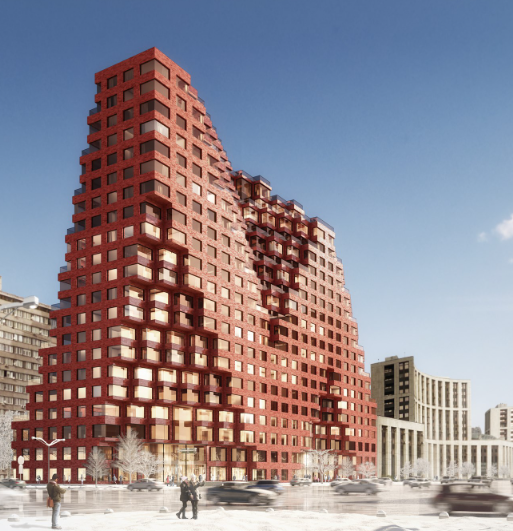
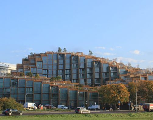
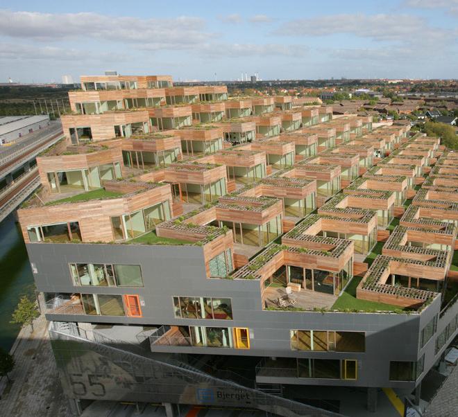
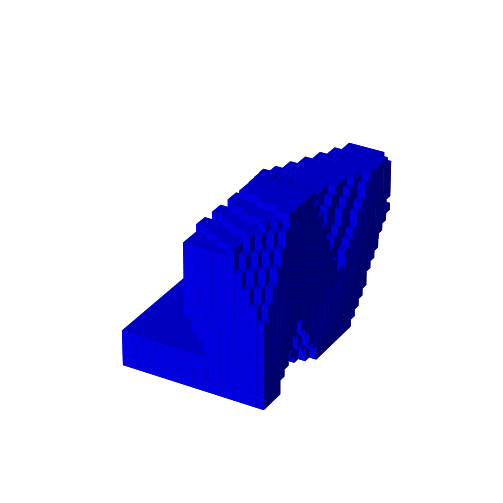
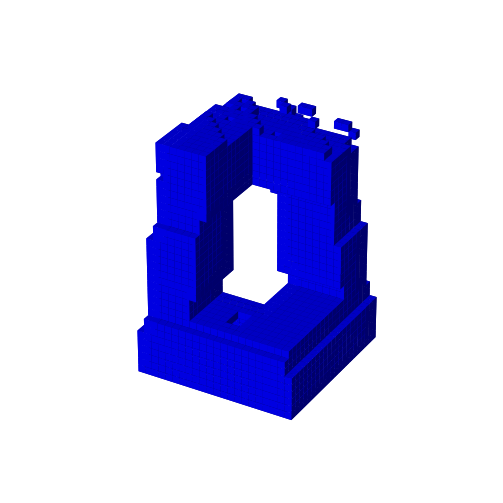
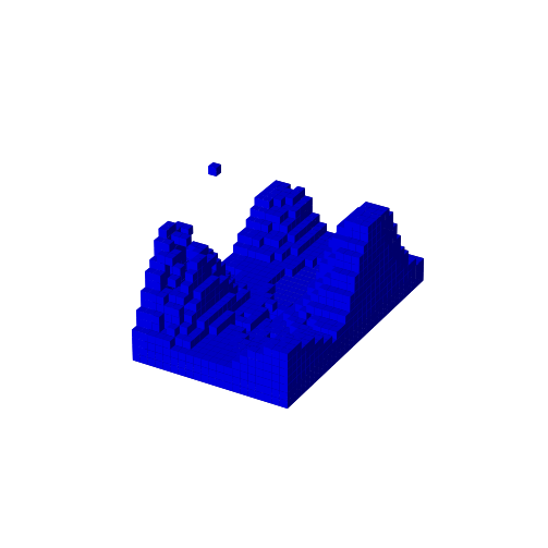
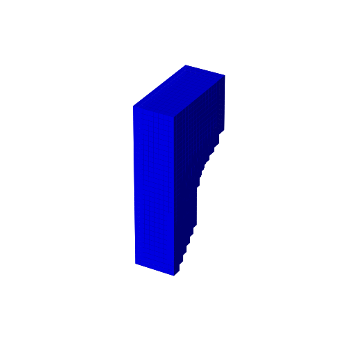
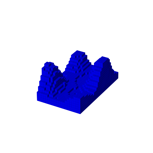
I collected building models designed by several famous architects for model training. The figure below shows the actual buildings from the modeling data I gathered.

Voxel-shaped buildings
From the left, RED7(MVRDV architects) · 79 and Park(BIG architects) · Mountain dwelling(BIG architects)

The buildings aforementioned possess a common characteristic: their voxel-shaped configuration. As stated above, we learned three modalities of 3D shape representations pertinent to GANs. The primary limitation of the voxel-shaped representation lies in its challenge to articulate high-resolution. However, within the realm of architectural design, this constraint might be reconceived as an opportunity. The voxel-shaped form is prevalently utilized in the architecture field, and there is no imperative demand for high-resolution depictions of such forms.

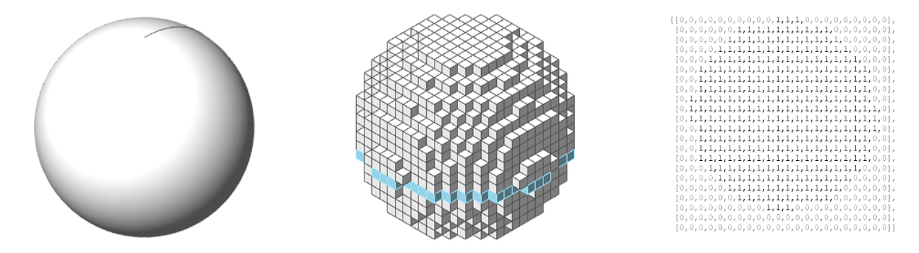
Therefore, we'll create a generative model that generates masses like to the aforementioned using voxel data with appropriate resolutions. Firstly, to train models utilizing modeling data, it is imperative to transform the data structure from the .obj format to the more suitable .binvox format. The .binvox format delineates data as a binary voxel grid structure, representing True (1) for solid regions and False (0) for vacant spaces. Let us look the illustrative example that is preprocessed to the .binvox format below.

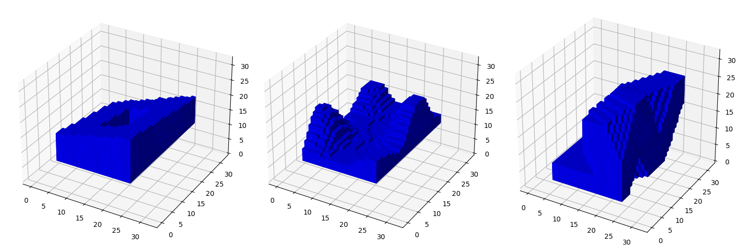
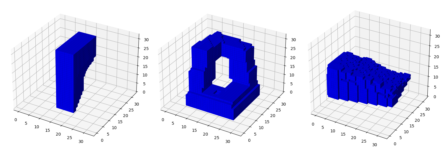
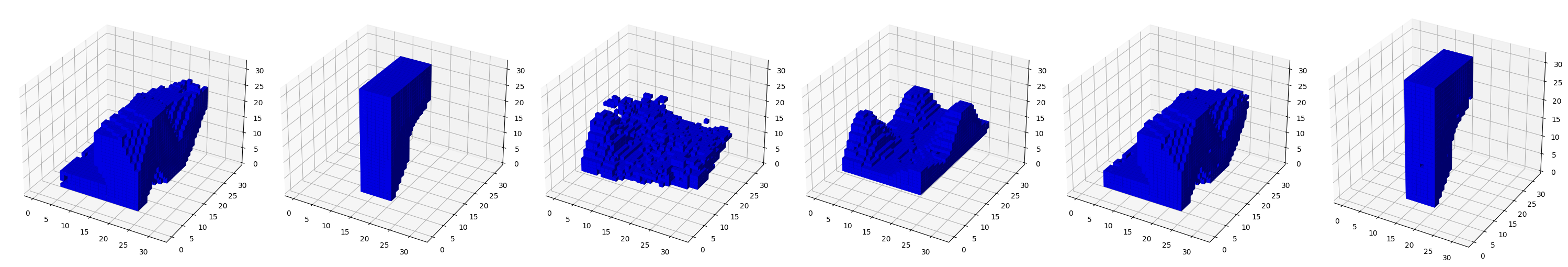
Binary voxel grid representations
From the left, Given sphere · Voxelated sphere · Binary voxel grid(9th voxels grid)
These were aforementioned in the part of my postings titled Voxelate

As stated above in the binary voxel grid, one can observe the vacant regions are represented by 0s, while the solid regions are denoted by 1s. All detailed code of preprocessing to the .binvox format is showing in the following link and I preprocessed to possess 32 x 32 x 32 resolution for 6 models below utilizing it.

Preprocessed data to the binary voxel grid utilizing binvox
From the top left, 79 and Park · Lego tower, RED7
From the bottom left, Vancouver house · CCTV Headquarter, Mountain dwelling

Implementation of models and training them

We have now completed the procedures for data collection and preprocessing. Subsequently, we are now poised to commence the implementation of both the generator and the discriminator.

Therefore I implemented DCGAN with a gradient penalty(WGAN) by referring to the GitHub repositories where several 3D generation models are implemented as follows. The comprehensive code delineating the model definitions can be accessed at the following link: massGAN/model.py


    class Generator(nn.Module, Config):
        def __init__(self, z_dim, init_out_channels: int = None):
            super().__init__()
            
            out_channels_0 = self.GENERATOR_INIT_OUT_CHANNELS if init_out_channels is None else init_out_channels
            out_channels_1 = int(out_channels_0 / 2)
            out_channels_2 = int(out_channels_1 / 2)

            self.main = nn.Sequential(
                nn.ConvTranspose3d(z_dim, out_channels_0, kernel_size=4, stride=1, padding=0, bias=False),
                nn.BatchNorm3d(out_channels_0),
                nn.ReLU(True),
                nn.ConvTranspose3d(out_channels_0, out_channels_1, kernel_size=4, stride=2, padding=1, bias=False),
                nn.BatchNorm3d(out_channels_1),
                nn.ReLU(True),
                nn.ConvTranspose3d(out_channels_1, out_channels_2, kernel_size=4, stride=2, padding=1, bias=False),
                nn.BatchNorm3d(out_channels_2),
                nn.ReLU(True),
                nn.ConvTranspose3d(out_channels_2, 1, kernel_size=4, stride=2, padding=1, bias=False),
                nn.Sigmoid()
            )
            
            self.to(self.DEVICE)
            
        def forward(self, x):
            return self.main(x)
        
        
    class Discriminator(nn.Module, Config):
        def __init__(self, init_out_channels: int = None):
            super().__init__()
            
            out_channels_0 = self.DISCRIMINATOR_INIT_OUT_CHANNELS if init_out_channels is None else init_out_channels
            out_channels_1 = out_channels_0 * 2
            out_channels_2 = out_channels_1 * 2

            self.main = nn.Sequential(
                nn.Conv3d(1, out_channels_0, kernel_size=4, stride=2, padding=1, bias=False),
                nn.LeakyReLU(0.2, inplace=True),
                nn.Conv3d(out_channels_0, out_channels_1, kernel_size=4, stride=2, padding=1, bias=False),
                nn.BatchNorm3d(out_channels_1),
                nn.LeakyReLU(0.2, inplace=True),
                nn.Conv3d(out_channels_1, out_channels_2, kernel_size=4, stride=2, padding=1, bias=False),
                nn.BatchNorm3d(out_channels_2),
                nn.LeakyReLU(0.2, inplace=True),
                nn.Conv3d(out_channels_2, 1, kernel_size=4, stride=1, padding=0, bias=False),
                nn.Sigmoid()
            )
            
            self.to(self.DEVICE)
            
        def forward(self, x):
            return self.main(x).view(-1, 1).squeeze(1)

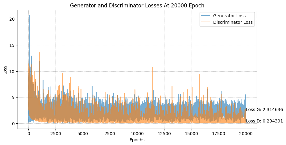
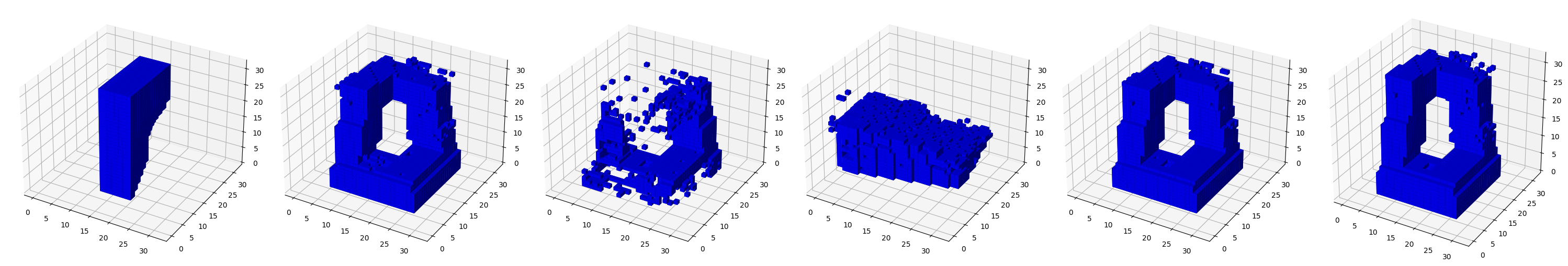
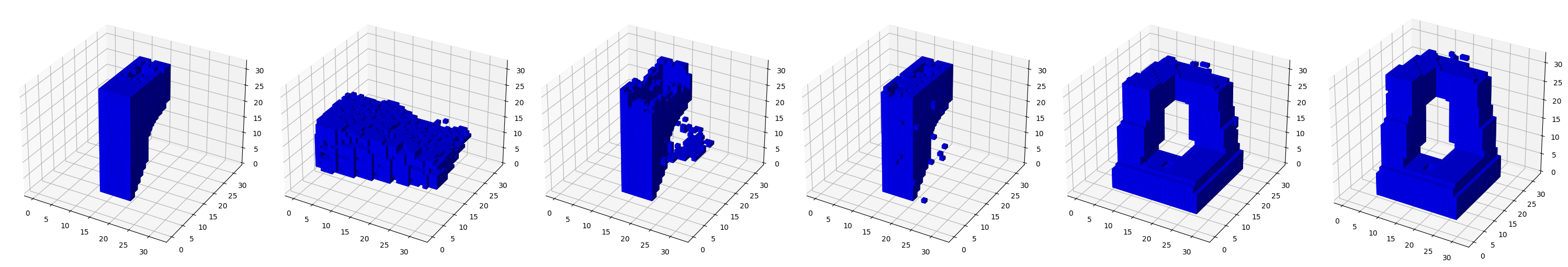
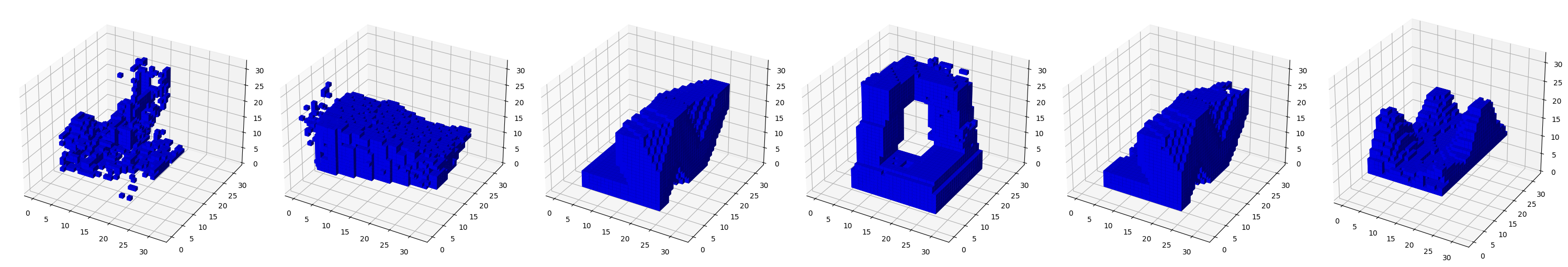
We further defined the MassganTrainer for model supervision, including model training, evaluation, and storage. Throughout this process, I monitored any issues that occurred during the training phase. The recorded outcomes are presented below:

Visualized training process at each 200 epochs from 0 to 20000
From the top, losses status · generated masses when training model

Contrary to the a single sphere GAN that we previously trained, MassGAN does not exhibit a loss value converging to a singular point due to the complexity of the data. Neverthelesee, if you compare the early and final stages of learning, you can observe that the loss value oscillates within a low range. Furthermore, by observing the monitored fake masses, one can discern that they progressively approximate the shapes of real masses.

Evaluating generator, and exploration for the latent spaces

The parameters for model training, such as learning rate, batch size, noise dimension, and so forth, were used as follows:


    class ModelConfig:
        """Configuration related to the GAN models
        """

        DEVICE = "cpu"
        if torch.cuda.is_available():
            DEVICE = "cuda"
            
        SEED = 777
        
        GENERATOR_INIT_OUT_CHANNELS = 256
        DISCRIMINATOR_INIT_OUT_CHANNELS = 64
        
        EPOCHS = 20000
        LEARNING_RATE = 0.0001
        BATCH_SIZE = 6
        BATCH_SIZE_TO_EVALUATE = 6
        Z_DIM = 128
        BETAS = (0.5, 0.999)
        
        LAMBDA_1 = 10
        
        LOG_INTERVAL = 200

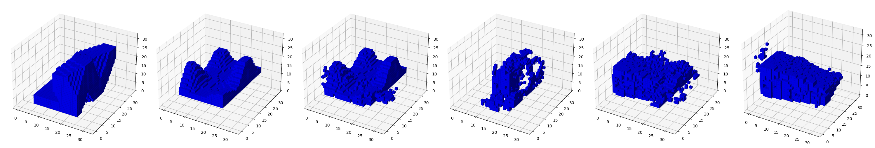
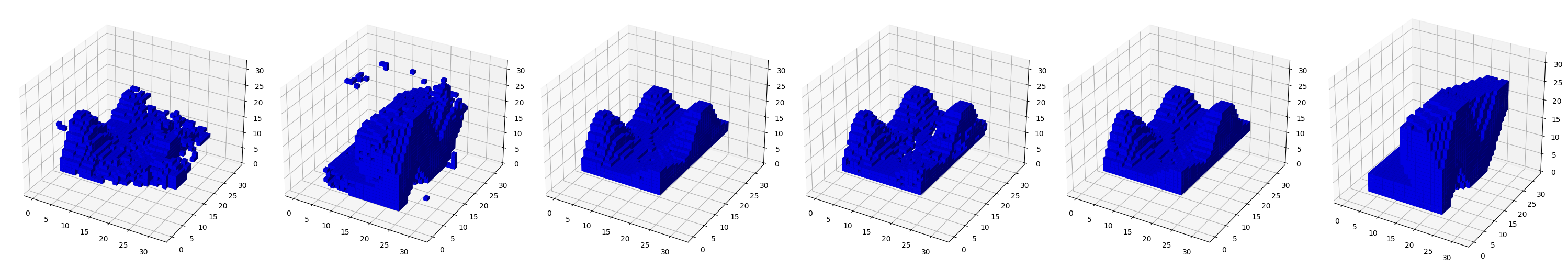
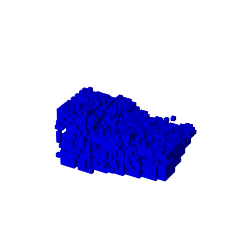
Now, let's load and evaluate the model trained with the corresponding ModelConfig. In GAN, it is important to evaluate the model quantitatively as the status of loss, but qualitatively evaluating the data generated by the Generator is also effective in evaluating the model. The following figures are generated masses by MassGAN model through the utilization of the evaluate function.

All in all, it appears to produce decent data. Subsequently, let's select some of the masses created by the generator and observe the interpolation of latent mass shapes between them.